Page 295 - Numerical Analysis Using MATLAB and Excel

Lagrange’s Interpolation Method

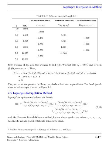
TABLE 7.11 Difference table for Example 7.6
1st Divided Difference 2nd Divided Difference 3rd Divided Difference

x fx() fx x,( 0 1 ) fx x x ) ( 0 , 1 , 2 fx x x x ) ( 0 , 1 , 2 , 3
−1.0 3.000
−5.000
0.0 −2.000 5.500
3.250 −1.000
0.5 −0.375 3.500
6.750 −1.000
1.0 3.000 1.000
8.750 −1.000
2.5 16.125 −1.500
5.750
3.0 19.000

*
Now, we have all the data that we need to find f2() . We start with x = 0.00 , and for in
x
0
(7.49), we use x = 2 . Then,
(
)
)
)
(
(
)
(
)
)
)
(
(
)
f2() = – 2.0 + ( 2 – 0 3.250 + ( 2 – 0 2 – 0.5 3.500 + ( 2 – 0 2 – 0.5 2 – 1 – 1.000 )
–
= – 2.0 + 6.5 + 10.5 3
= 12
This, and other interpolation problems, can also be solved with a spreadsheet. The Excel spread-
sheet for this example is shown in Figure 7.1.
7.5 Lagrange’s Interpolation Method
Lagrange’s interpolation method uses the formula
( x – x ) ( xx ) – … ( x – x ) ( xx ) – ( x – x ) … ( xx ) –
0
1
n
2
n
2
fx() = ------------------------------------------------------------------------fx ( ) + ------------------------------------------------------------------------fx ( )
( x – x ) 1 ( x – x ) 2 … ( x – x ) n 0 ( x – x ) 0 ( x – x ) 2 … ( x – x ) n 1
0
0
1
1
1
0
( x – x ) ( xx ) – … ( x – x ) (7.53)
n –
1
1
0
+ ------------------------------------------------------------------------------fx ( )
( x – x ) 0 ( x – x ) 2 … ( x – x n – 1 ) n
n
n
n
and, like Newton’s divided difference method, has the advantage that the values x x x … x, 0 1 , 2 , , n
need not be equally spaced or taken in consecutive order.
* We chose this as our starting value so that f2() will be between f1() and f2.5 )
(
Numerical Analysis Using MATLAB® and Excel®, Third Edition 7−17
Copyright © Orchard Publications