Page 296 - Numerical Methods for Chemical Engineering

Discretized PDEs with more than two spatial dimensions 285

a

1 1

1 1

2 2
1 1 2 1 1 2
n 12 n 1
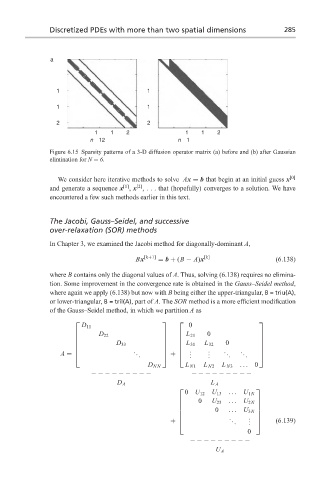
Figure 6.15 Sparsity patterns of a 3-D diffusion operator matrix (a) before and (b) after Gaussian
elimination for N = 6.

We consider here iterative methods to solve Ax = b that begin at an initial guess x [0]
[2]
[1]
and generate a sequence x , x ,... that (hopefully) converges to a solution. We have
encountered a few such methods earlier in this text.

The Jacobi, Gauss–Seidel, and successive
over-relaxation (SOR) methods

In Chapter 3, we examined the Jacobi method for diagonally-dominant A,

Bx [k+1] = b + (B − A)x [k] (6.138)

where B contains only the diagonal values of A. Thus, solving (6.138) requires no elimina-
tion. Some improvement in the convergence rate is obtained in the Gauss–Seidel method,
where again we apply (6.138) but now with B being either the upper-triangular, B = triu(A),
or lower-triangular, B = tril(A), part of A. The SOR method is a more efficient modification
of the Gauss–Seidel method, in which we partition A as

   
D 11 0
0
 L 21
D 22
  
   
   0 
D 33 L 31 L 32
   
 .

 . .  +  . . . . . . . 
A =  . . . . . 
D NN L N1 L N2 L N3 ... 0
−−−−−−−−− −−−−−−−−−
D A L A
 
0 U 12 U 13 ... U 1N
0
 U 23 ... U 2N 
 
 0 
 ... U 3N 
.
 . . 
+  . . .  (6.139)
0
−−−−−−−−−
U A