Page 295 - Numerical Methods for Chemical Engineering

284 6 Boundary value problems

1
nn A
nn
1
er eeents

1

ner nn 1

1 2
1 11 12 1 1 1

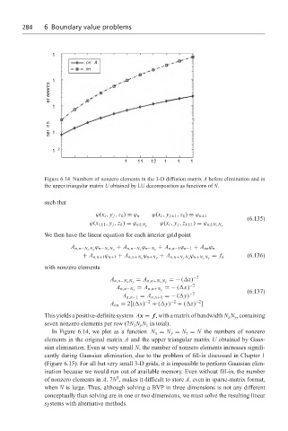
Figure 6.14 Numbers of nonzero elements in the 3-D diffusion matrix A before elimination and in
the upper triangular matrix U obtained by LU decomposition as functions of N.

such that

ϕ(x i , y j , z k ) = ϕ n ϕ(x i , y j±1 , z k ) = ϕ n±1
(6.135)
ϕ(x i±1 , y j , z k ) = ϕ n±N y ϕ(x i , y j , z k±1 ) = ϕ n±N x N y
We then have the linear equation for each interior grid point

ϕ ϕ
A n,n−N x N y n−N x N y + A n,n−N y n−N y + A n,n−1 ϕ n−1 + A nn ϕ n
ϕ ϕ (6.136)
+ A n,n+1 ϕ n+1 + A n,n+N y n+N y + A n,n+N x N y n+N x N y = f n
with nonzero elements
=− ( z) −2
A n,n−N x N y = A n,n+N x N y
=− ( x) −2
A n,n−N y = A n,n+N y (6.137)
A n,n−1 = A n,n+1 =− ( y) −2
−2
A nn = 2[( x) −2 + ( y) −2 + ( z) ]
This yields a positive-definite system Ax = f , with a matrix of bandwidth N x N y , containing
seven nonzero elements per row (7N x N y N z in total).
In Figure 6.14, we plot as a function N x = N y = N z = N the numbers of nonzero
elements in the original matrix A and the upper triangular matrix U obtained by Gaus-
sian elimination. Even at very small N, the number of nonzero elements increases signifi-
cantly during Gaussian elimination, due to the problem of fill-in discussed in Chapter 1
(Figure 6.15). For all but very small 3-D grids, it is impossible to perform Gaussian elim-
ination because we would run out of available memory. Even without fill-in, the number
3
of nonzero elements in A,7N , makes it difficult to store A, even in sparse-matrix format,
when N is large. Thus, although solving a BVP in three dimensions is not any different
conceptually than solving are in one or two dimensions, we must solve the resulting linear
systems with alternative methods.