Page 294 - Numerical Methods for Chemical Engineering

Discretized PDEs with more than two spatial dimensions 283

2 1

1 arrws sw
evtin
A 1 B crves wit
increasin
tie
2

1 1

2 2

1 1

1 1

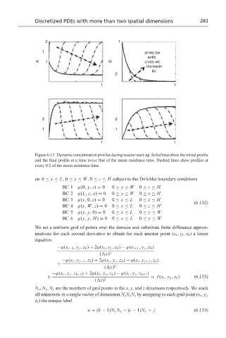
Figure 6.13 Dynamic concentration profiles during reactor start-up. Solid lines show the initial profile
and the final profile at a time twice that of the mean residence time. Dashed lines show profiles at
every 0.2 of the mean residence time.

on 0 ≤ x ≤ L, 0 ≤ y ≤ W, 0 ≤ z ≤ H subject to the Dirichlet boundary conditions
BC 1 ϕ(0, y, z) = 0 0 ≤ y ≤ W 0 ≤ z ≤ H
BC 2 ϕ(L, y, z) = 0 0 ≤ y ≤ W 0 ≤ z ≤ H
BC 3 ϕ(x, 0, z) = 0 0 ≤ x ≤ L 0 ≤ z ≤ H
(6.132)
BC 4 ϕ(x, W, z) = 0 0 ≤ x ≤ L 0 ≤ z ≤ H
BC 5 ϕ(x, y, 0) = 0 0 ≤ x ≤ L 0 ≤ y ≤ W
BC 6 ϕ(x, y, H) = 00 ≤ x ≤ L 0 ≤ y ≤ W
We set a uniform grid of points over the domain and substitute finite difference approx-
imations for each second derivative to obtain for each interior point (x i , y j , z k ) a linear
equation
−ϕ(x i−1 , y j , z k ) + 2ϕ(x i , y j , z k ) − ϕ(x i+1 , y j , z k )
( x) 2
−ϕ(x i , y j−1 , z k ) + 2ϕ(x i , y j , z k ) − ϕ(x i , y j+1 , z k )
+
( y) 2
−ϕ(x i , y j , z k−1 ) + 2ϕ(x i , y j , z k ) − ϕ(x i , y j , z k+1 )
+ = f (x i , y j , z k ) (6.133)
( z) 2
N x , N y , N z are the numbers of grid points in the x, y, and z directions respectively. We stack
all unknowns in a single vector of dimension N x N y N z by assigning to each grid point (x i , y j ,
z k ) the unique label

n = (k − 1)N x N y + (i − 1)N y + j (6.134)