Page 292 - Numerical Methods for Chemical Engineering

Modeling a tubular chemical reactor with dispersion 281

cee cee

1
1
1
1
2
2
1 1 2 1 1 2
n 112 n 112
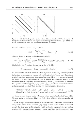
Figure 6.11 Effect of stacking on the sparsity pattern of the Jacobian for a BVP involving the 1-D
transport of four fields, with local coupling of each field through the source terms. A grid of 50 points
is used to discretize the PDEs. Plot generated by BVP field JPattern.m.

From the inlet boundary condition, we obtain
Pe loc c j0 + c j (z 1 ) v z z 1
c j (z 0 ) = Pe loc = (6.125)
1 + Pe loc D
Thus, for k = 1 we have the modified version of (6.122),

α lo α lo Pe loc c j0
0 = α mid + c j (z 1 ) + + α hi c j (z 2 ) + s j [{c m (z 1 )}] (6.126)
1 + Pe loc 1 + Pe loc
Similarly, for k = N we have the modified version of (6.122),

0 = α lo c j (z N−1 ) + [α mid + α hi ]c j (z N ) + s j [{c m (z N )}] (6.127)

We now stack the set of all unknowns into a single state vector using a labeling system
that assigns to each unknown a unique integer. Equation (6.122) forms a set of nonlinear
algebraic equations with a sparse Jacobian, and thus to avoid the fill-in problems discussed
in Chapter 1, we make the bandwidth as small as possible (i.e., cluster the nonzero values
around the principal diagonal). We see that (6.122) relates c j (z k ), the values of the same
field c j at the neighboring points, c j (z k−1 ) and c j (z k+1 ), and the values of all other fields
at the same point, c m = j (z k ). Thus, from the two ways to stack the state vector,
T
Scheme I x = [c A (z 1 ) c A (z 2 ) ··· c A (z N ) c B (z 1 ) ··· c B (z N ) ··· c D (z N )]
(6.128)
T
Scheme II x = [c A (z 1 ) c B (z 1 ) c C (z 1 ) c D (z 1 ) c A (z 2 ) c B (z 2 ) ··· c C (z N ) c D (z N )]
we choose scheme II, as it yields a Jacobian with a smaller bandwidth (Figure 6.11).
We thus assign to c j (z k ) the label n = N f (k − 1) + j, N f = 4 being the number of
fields.
When coding a BVP with multiple fields, it is easiest to write the routines to use, as much
as is possible, natural names and indices, e.g. c j (z k ), and to rely upon routines to stack and
unstack the state vector and to place the matrix and vector elements in the appropriate
positions. This approach is used in tubular reactor 2rxn SS.m. Sample results are shown