Page 290 - Numerical Methods for Chemical Engineering

Modeling a tubular chemical reactor with dispersion 279

cte cncentratins c (z)
j
inet A + B → C r R1 = k c c tet
1 A B
C + B → D r R2 = k c c
2 B C
z = 0 z = L
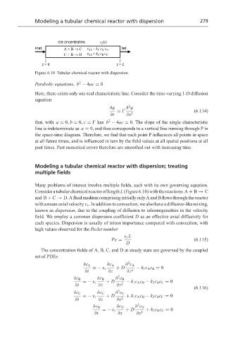
Figure 6.10 Tubular chemical reactor with dispersion.

2
Parabolic equations, b − 4ac = 0
Here, there exists only one real characteristic line. Consider the time-varying 1-D diffusion
equation
2
∂ϕ ∂ ϕ
= (6.114)
∂t ∂z 2
2
that, with a = 0, b = 0, c = has b − 4ac = 0. The slope of the single characteristic
line is indeterminate as a = 0, and thus corresponds to a vertical line running through P in
the space-time diagram. Therefore, we find that each point P influences all points in space
at all future times, and is influenced in turn by the field values at all spatial positions at all
past times. Past numerical errors therefore are smoothed out with increasing time.

Modeling a tubular chemical reactor with dispersion; treating
multiple fields

Many problems of interest involve multiple fields, each with its own governing equation.
Consider a tubular chemical reactor of length L (Figure 6.10) with the reactions A + B → C
and B + C → D.AfluidmediumcomprisinginitiallyonlyAandBflowsthroughthereactor
with a mean axial velocity v z . In addition to convection, we also have a diffusive-like mixing,
known as dispersion, due to the coupling of diffusion to inhomogeneities in the velocity
field. We employ a common dispersion coefficient D as an effective axial diffusivity for
each species. Dispersion is usually of minor importance compared with convection, with
high values observed for the Peclet number
v z L
Pe = (6.115)
D
The concentration fields of A, B, C, and D at steady state are governed by the coupled
set of PDEs
2
∂c A ∂c A ∂ c A
=− v z + D − k 1 c A c B = 0
∂t ∂z ∂z 2
2
∂c B ∂c B ∂ c B
=− v z + D 2 − k 1 c A c B − k 2 c B c C = 0
∂t ∂z ∂z
(6.116)
2
∂c C ∂c C ∂ c C
=− v z + D + k 1 c A c B − k 2 c B c C = 0
∂t ∂z ∂z 2
2
∂c D ∂c D ∂ c D
=− v z + D 2 + k 2 c B c C = 0
∂t ∂z ∂z