Page 293 - Numerical Methods for Chemical Engineering

282 6 Boundary value problems

1
A
B

secies cncentratins

2
1

2 1

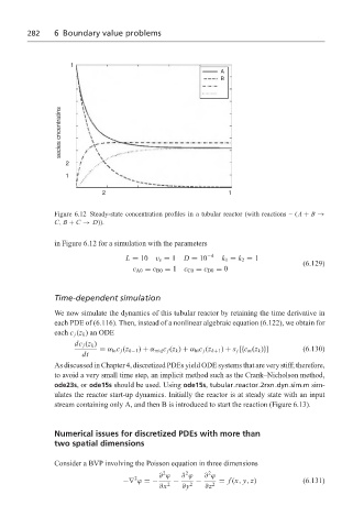
Figure 6.12 Steady-state concentration profiles in a tubular reactor (with reactions – (A + B →
C, B + C → D)).

in Figure 6.12 for a simulation with the parameters
L = 10 v z = 1 D = 10 −4 k 1 = k 2 = 1
(6.129)
c A0 = c B0 = 1 c C0 = c D0 = 0

Time-dependent simulation
We now simulate the dynamics of this tubular reactor by retaining the time derivative in
each PDE of (6.116). Then, instead of a nonlinear algebraic equation (6.122), we obtain for
each c j (z k )anODE
dc j (z k )
= α lo c j (z k−1 ) + α mid c j (z k ) + α hi c j (z k+1 ) + s j [{c m (z k )}] (6.130)
dt
As discussed in Chapter 4, discretized PDEs yield ODE systems that are very stiff; therefore,
to avoid a very small time step, an implicit method such as the Crank–Nicholson method,
ode23s,or ode15s should be used. Using ode15s, tubular reactor 2rxn dyn sim.m sim-
ulates the reactor start-up dynamics. Initially the reactor is at steady state with an input
stream containing only A, and then B is introduced to start the reaction (Figure 6.13).

Numerical issues for discretized PDEs with more than
two spatial dimensions

Consider a BVP involving the Poisson equation in three dimensions
2
2
2
∂ ϕ ∂ ϕ ∂ ϕ
2
−∇ ϕ =− − − = f (x, y, z) (6.131)
∂x 2 ∂y 2 ∂z 2