Page 355 - Numerical Methods for Chemical Engineering

344 7 Probability theory and stochastic simulation

∆t 1 ∆t 1

2 2
t t

−2 −2
− −
1 1
t t
∆t 1 ∆t 1

2 2

1 1
t t

−1 −1
−2 −2
1 1
t t
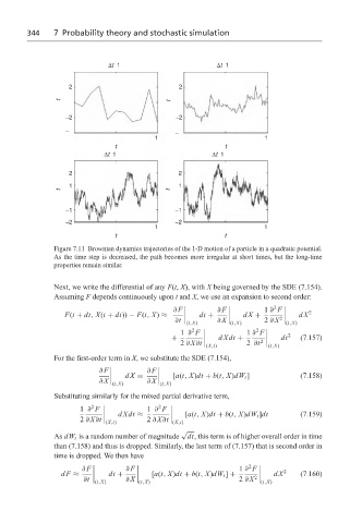
Figure 7.11 Brownian dynamics trajectories of the 1-D motion of a particle in a quadratic potential.
As the time step is decreased, the path becomes more irregular at short times, but the long-time
properties remain similar.

Next, we write the differential of any F(t, X), with X being governed by the SDE (7.154).
Assuming F depends continuously upon t and X, we use an expansion to second order:
2

∂F ∂ F 1 ∂ F 2
F(t + dt, X(t + dt)) − F(t, X) ≈ dt + dX + dX
∂t ∂ X 2 ∂ X 2
(t,X) (t,X) (t,X)
2 2
1 ∂ F 1 ∂ F 2
+ dXdt + dt (7.157)
2 ∂ X∂t 2 ∂t 2
(X,t) (t,X)
For the first-order term in X, we substitute the SDE (7.154),

∂F ∂F
dX = [a(t, X)dt + b(t, X)dW t ] (7.158)
∂ X ∂ X
(t,X) (t,X)
Substituting similarly for the mixed partial derivative term,
2 2
1 ∂ F 1 ∂ F
dXdt ≈ [a(t, X)dt + b(t, X)dW t ]dt (7.159)
2 ∂ X∂t 2 ∂ X∂t
(X,t) (X,t)
√
As dW t is a random number of magnitude dt, this term is of higher overall order in time
than (7.158) and thus is dropped. Similarly, the last term of (7.157) that is second order in
time is dropped. We then have
2

∂ F ∂F 1 ∂ F 2
dF ≈ dt + [a(t, X)dt + b(t, X)dW t ] + dX (7.160)
∂t ∂ X 2 ∂ X 2
(t,X) (t,X) (t,X)