Page 358 - Numerical Methods for Chemical Engineering

Brownian dynamics and SDEs 347

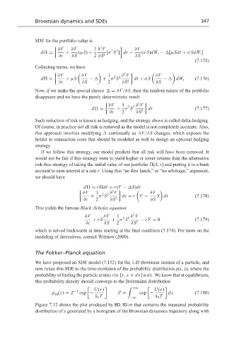
SDE for the portfolio value is
∂V ∂V 1 ∂ V 2 2 ∂V
2 1
d = + (µS) + [σ S ] dt + (σ S)dW t − [µSdt + σ SdW t ]
∂t ∂S 2 ∂S 2 ∂S
(7.175)
Collecting terms, we have
∂V ∂V 1 2 2 ∂ V ∂V
2 1
d = + µS − + σ S dt + σ S − dW t (7.176)
∂t ∂S 2 ∂S 2 ∂S
Now, if we make the special choice = ∂V/∂S, then the random nature of the portfolio
disappears and we have the purely deterministic result

∂V 1 2 2 ∂ V
2 1
d = + σ S dt (7.177)
∂t 2 ∂S 2
Such reduction of risk is known as hedging, and the strategy above is called delta-hedging.
Of course, in practice not all risk is removed as the model is not completely accurate. Also,
this approach involves modifying continually as ∂V/∂S changes, which exposes the
holder to transaction costs that should be modeled as well to design an optional hedging
strategy.
If we follow this strategy, our model predicts that all risk will have been removed. It
would not be fair if this strategy were to yield higher or lower returns than the alternative
risk-free strategy of taking the initial value of our portfolio (S, t) and putting it in a bank
account to earn interest at a rate r. Using this “no free lunch,” or “no arbitrage,” argument,
we should have

d = r dt = r(V − S)dt
2 1
∂V 1 2 2 ∂ V ∂V
+ σ S dt = r V − S dt (7.178)
∂t 2 ∂S 2 ∂S
This yields the famous Black–Scholes equation
2
∂V ∂V 1 2 2 ∂ V
+ rS + σ S − rV = 0 (7.179)
∂t ∂S 2 ∂S 2
which is solved backwards in time starting at the final condition (7.174). For more on the
modeling of derivatives, consult Wilmott (2000).

The Fokker–Planck equation

We have proposed an SDE model (7.152) for the 1-D Brownian motion of a particle, and
now relate this SDE to the time-evolution of the probability distribution p(t, x), where the
probability of finding the particle at time t in [x, x + dx]is dx. We know that at equilibrium,
this probability density should converge to the Boltzmann distribution
U(x) U(x)
' +∞
−1
p eq (x) = Z exp − Z = exp − dx (7.180)
k b T k b T
−∞
Figure 7.12 shows the plot produced by BD 1D.m that contains the measured probability
distribution of x generated by a histogram of the Brownian dynamics trajectory along with