Page 359 - Numerical Methods for Chemical Engineering

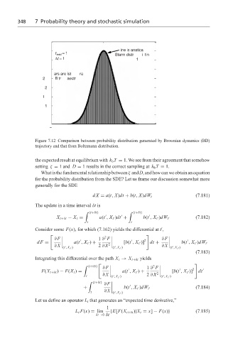
348 7 Probability theory and stochastic simulation

ine is anatica
t end = 1 Btann distr i tin
∆t = 1 1

ars are ist ra
2 B tr aectr
2
1

1

−

Figure 7.12 Comparison between probability distribution generated by Brownian dynamics (BD)
trajectory and that from Boltzmann distribution.

the expected result at equilibrium with k b T = 1. We see from their agreement that somehow
setting ζ = 1 and D = 1 results in the correct sampling at k b T = 1.
Whatisthefundamentalrelationshipbetweenζ andD,andhowcanweobtainanequation
for the probability distribution from the SDE? Let us frame our discussion somewhat more
generally for the SDE

(7.181)
dX = a(t, X)dt + b(t, X)dW t
The update in a time interval δt is
(t+δt) (t+δt)
' '

X t+δt − X t = a(t , X t )dt + b(t , X t )dW t (7.182)

t t

Consider some F(x), for which (7.162) yields the differential at t ,

2

∂ F 1 ∂ F 2 ∂ F

dF = a(t , X t ) + [b(t , X t )] dt + b(t , X t )dW t

∂ X 2 ∂ X 2 ∂ X
(t ,X t ) (t ,X t ) (t ,X t )

(7.183)
Integrating this differential over the path X t → X t+δt yields

' (t+δt) 2
∂ F 1 ∂ F 2

F(X t+δt ) − F(X t ) = a(t , X t ) + [b(t , X t )] dt

t ∂ X (t ,X t ) 2 ∂ X 2 (t ,X t )

' (t+δt)
∂F
+ b(t , X t )dW t (7.184)

∂ X
t (t ,X t )

Let us define an operator L t that generates an “expected time derivative,”
1
L t F(x) = lim {E[F(X t+δt )|X t = x] − F(x)} (7.185)
δt→0 δt