Page 414 - Offshore Electrical Engineering Manual

Confidence Limits 401

Various statistics may be calculated from the data available. Those of particular
interest here are as follows. First, the sample variance is given by
2
2
2
2
s = (x 1 − x) + (x 2 − x) +⋯ + (x n − x) / (n − 1)
The sample standard deviation s is obtained by taking the square root of the vari-
ance. The true population variance is usually denoted by σ.
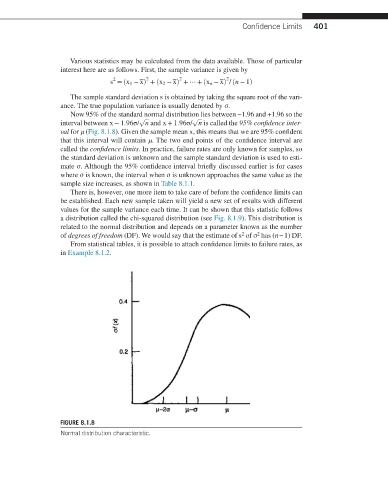
Now 95% of the standard normal distribution lies between −1.96 and +1.96 so the
√
√
interval between x − 1.96σ/ n and x + 1.96σ/ n is called the 95% confidence inter-
val for μ (Fig. 8.1.8). Given the sample mean x, this means that we are 95% confident
that this interval will contain μ. The two end points of the confidence interval are
called the confidence limits. In practice, failure rates are only known for samples, so
the standard deviation is unknown and the sample standard deviation is used to esti-
mate σ. Although the 95% confidence interval briefly discussed earlier is for cases
where σ is known, the interval when σ is unknown approaches the same value as the
sample size increases, as shown in Table 8.1.1.
There is, however, one more item to take care of before the confidence limits can
be established. Each new sample taken will yield a new set of results with different
values for the sample variance each time. It can be shown that this statistic follows
a distribution called the chi-squared distribution (see Fig. 8.1.9). This distribution is
related to the normal distribution and depends on a parameter known as the number
2
2
of degrees of freedom (DF). We would say that the estimate of s of σ has (n − 1) DF.
From statistical tables, it is possible to attach confidence limits to failure rates, as
in Example 8.1.2.

FIGURE 8.1.8
Normal distribution characteristic.