Page 340 - Orlicky's Material Requirements Planning

CHAPTER 19 Repetitive Manufacturing Application 319

ed or stopped until the supplier is able to provide the needed part. There is insufficient
response time for the supplier to react to a requirement that blindsides him or her. If a
supplier has been delivering blue parts at a constant rate and then, all of a sudden, a kan-
ban shows up with a demand for a striped part, the chance that the striped part will be
available is very small without having some forewarning that the demand is coming.
This is why an MRP system still has an integral place in a repetitive manufacturing busi-
ness. MRP can very effectively plan to the day exactly what is required and when.
Practically speaking, most facilities find a daily schedule to be sufficient to support pro-
duction. Rarely can an enterprise schedule and react to the hour or exact time. The kan-
ban then can become the execution tool of less than one day’s duration with the exact tim-
ing of the replenishment when production is ready.

RATE-BASED SCHEDULING
Rate-based scheduling occurs when a production schedule is entered directly into the
system as a date range with volumes. The following could be an example of a rate-based
schedule:

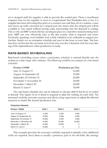
Product 135948 Production per Day
June 10–August 15 12,000
August 16–September 22 15,000
September 23–October 31 20,000
November 1–November 30 30,000
December 1–March 30 20,000
March 31–June 9 10,000
The rate-based schedule also can be entered as rate per shift if that level of control
is desired. This higher level of detail is required to plan the staffing for each shift. The
increased visibility prevents surprises and allows shop supervisors to adjust the affected
resources to match the desired production rate.

Production Schedule
Product 135948 Shift 1 Shift 2 Shift 3

June 10–August 15 6,000 3,000 3,000
August 16–September 22 10,000 3,000 2,000
September 23–October 31 10,000 5,000 5,000
November 1–November 30 10,000 10,000 10,000
December 1–March 30 10,000 10,000 0
March 31–June 9 10,000 0 0

This example provides the necessary visibility required to identify when additional
shifts are required. Since there is usually a premium paid to the off-shifts, the strategy