Page 342 - Orlicky's Material Requirements Planning

CHAPTER 19 Repetitive Manufacturing Application 321

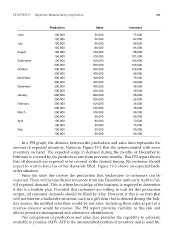
Production Sales Inventory

June 100,000 50,000 75,000
120,000 50,000 82,000
July 120,000 60,000 88,000
120,000 60,000 94,000
August 120,000 100,000 96,000
150,000 100,000 101,000
September 150,000 100,000 106,000
200,000 200,000 106,000
October 200,000 200,000 106,000
200,000 400,000 86,000
November 300,000 400,000 76,000
300,000 400,000 66,000
December 200,000 400,000 46,000
200,000 400,000 26,000
January 200,000 200,000 26,000
200,000 200,000 26,000
February 200,000 100,000 36,000
200,000 100,000 46,000
March 200,000 100,000 56,000
200,000 80,000 68,000
April 100,000 80,000 70,000
100,000 50,000 75,000
May 100,000 50,000 80,000
100,000 50,000 85,000

In a PSI graph, the distance between the production and sales lines represents the
amount of expected inventory. Notice in Figure 19-2 that the system started with some
inventory on hand. The expected surge in demand during the months of December to
February is covered by the production rate from previous months. This PSI report shows
that all demands are expected to be covered at the desired timing. No customer should
expect to wait to have his or her demands filled. Figure 19-3 shows an expected back -
order situation.
Since the sales line crosses the production line, backorders to customers can be
expected. There will be insufficient inventory from late December until early April to ful-
fill expected demand. This is where knowledge of the business is required to determine
if this is a feasible plan. Provided that customers are willing to wait for this production
output, all customer demands should be filled by May. However, if this is an item that
will not tolerate a backorder situation, such as a gift item that is desired during the holi-
day season, the unfilled sales then would be lost sales. Including these sales as part of a
revenue forecast would be unwise. The PSI report provides visibility to this risk and
allows proactive management and alternative identification.
The comparison of production and sales also provides the capability to calculate
available to promise (ATP). ATP is the uncommitted portion of inventory and is used fre-