Page 22 - Percolation Models for Transport in Porous Media With

1.2 RANDOM CONDUCTNITIES 13

characterized by the normalized radius distribution function of conducting bonds
f(r). From now on, a corresponding form of function u(r) will be used for specific
transfer phenomena, and the function /(r) will be used to describe heterogeneity
of the porous medium. Within this section of the book, for clarity's sake, we shall
use f 0(u) in our reasoning. Let the number of bonds with conductivities u > 0
be characterized by the quantity ~~:(0 $ ~~: $ 1). Here~~:= 1 only if all bonds are
conducting and 0 $ ~~: < 1 otherwise. Conduct a mental experiment. Suppose that
the bond conductivities with values less than u1 vanish. Then percolation is pos-
sible only through those bonds, whose conductivities exceed u1 • The probability
of a bond having conductivity u ~ u1 is

00 00
Pb(u1(r1)) = 11: I fo(u) da = ~~: I f(r) dr, (1.7)

CTl rt(crt)
where r1 (ut) is the inverse relation o-1 (r1). The infinite cluster and, consequently,
percolation appears in the network when pb(ut) ~ P:. Using relationships {1.1)
and (1.7), one can find the value uc(rc) of conductivity at the point when the IC
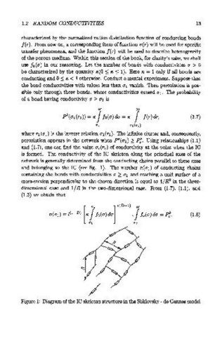
is formed. The conductivity of the IC skeleton along the principal axes of the
network is generally determined from the conducting chains parallel to these axes
and belonging to the IC (see fig. 1). The number n(ut) of conducting chains
containing the bonds with conductivities u ~ u1 and reaching a unit surface of a
cross-section perpendicular to the chosen direction is equal to 1/ R 2 in the three-
dimensional case and 1/R in the two-dimensional case. From (1.7), (1.1), and
(1.3) we obtain that

/

Figure 1: Diagram of the IC skeleton structure in the Shklovsky- de Gennes model