Page 25 - Percolation Models for Transport in Porous Media With

16 CHAPTER 1. PERCOLATION MODEL

i•l,j-1 i•l,j i•l,j•l

i+I/Z,j i•I/Z,j•l
i,j-1/2 ~j·l/2
i,j-1 i.j
i-1/Z,j

·-1, . _, i-1, .
l J j i·!,j•l
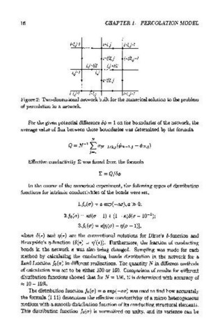
Figure 2: Two-dimensional network built for the numerical solution to the problem
of percolation in a network.

For the given potential difference 6¢ = 1 on the boundaries of the network, the
average value of flux between those boundaries was determined by the formula
N
1
Q = N- LO'N-1/2,j(¢N-l.j- ¢N,j)
j=1
Effective conductivity E was found from the formula
E = Q/6¢

In the course of the numerical experiment, the following types of distribution
functions for intrinsic conductivities of the bonds were set,

1./o(a) =a exp( -aa), a:» 0;

1
2./o(a) =~(a -1) + (1- K.)6(a -10- );
3.fo(a) = K.[17(a) - 17(a- 1)],

where 6(*) and 77(*) are the conventional notations for Dirac's 6-function and
Heavyside's 77-function (6(*) = 77'(*)). Furthermore, the fraction of conducting
bonds in the network K. was also being changed. Sampling was made for each
method by calculating the conducting bonds distribution in the network for a
fixed function f 0 (a) in different realizations. The quantity N in different methods
of calculation was set to be either 100 or 150. Comparison of results for different
distribution functions showed that for N = 150, E is determined with accuracy of
~ 10-15%.
The distribution function f 0(a) =a exp( -aa) was used to find how accurately
the formula (1.11) determines the effective conductivity of a micro heterogeneous
medium with a smooth distribution function of its conducting structural elements.
This distribution function f 0 (a) is normalized on unity, and its variance can be