Page 26 - Percolation Models for Transport in Porous Media With

1.2 RANDOM CONDUCTIVITIES 17

I: E
a 1,0 I
.1
0,8 I
I
D,6 X I I
I
0,+ I
I
·-· / /
IJ,l .,. I
/
D 0,2 0,~ 11,6 0,8 1,0 D 42 41- 4$ 0,1 f,D
c z

0,¥

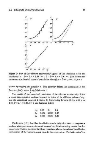
Figure 3: Plot of the effective conductivity against of the parameter K for the
conditions: a- D = 2,11 = 1.33, l = 1; b- D = 3,11 = 0.9, l = 1 (the dotted line
represents the classical curve of percolation theory); c- D = 2,11 = 1.33, l = 1

altered by varying the quantity a. This quantity defines the expectation of the
00
function /o(a): mt = J afo(a)da = a- 1 .
0
The results of the numerical calculation of the effective conductivity E for
a micro heterogeneous medium (marked by index p) for different values of mf,
and the theoretical values of E (index t), found using formula (1.11), with 11 =
1.33, D = 2,1 = 2.85, l = 1, are displayed below:

0.05 0.1 0.5
0.043 0.089 0.47
0.043 0.088 0.45

The formula (1.11) describes the effective conductivity of a micro heterogeneous
medium with good accuracy in a wide range of m 1. It is interesting to note that for
smooth distribution functions like those considered above, the value of the effective
conductivity of the network comes close to the expectation. The latter coincides