Page 147 - Phase Space Optics Fundamentals and Applications

128 Chapter Four

Exit pupil
Focal plane
y
Observation
point
x
α φ o
a (z + f ) tanα

Σ P f
z

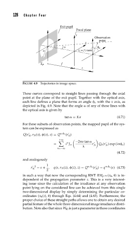
FIGURE 4.9 Trajectories in image space.

These curves correspond to straight lines passing through the axial
point at the plane of the exit pupil. Together with the optical axis,
each line defines a plane that forms an angle o with the x axis, as
depicted in Fig. 4.9. Note that the angle of any of these lines with
the optical axis is given by

tan = Ka (4.71)
For these subsets of observation points, the mapped pupil of the sys-
tem can be expressed as

Q(r ,r N (z), (z),z) = Q , o (r )
N N
+∞
, −2 a tan
n
= i J n r N Q n (r ) exp (in o )
N

n=−∞
(4.72)
and analogously
1

r 2 = s + , q(s, r N (z), (z),z) = Q , o (r ) = q , o (s) (4.73)
N N
2
, o (x , ) is in-
in such a way that now the corresponding RWT RW q
dependent of the propagation parameter z. This is a very interest-
ing issue since the calculation of the irradiance at any observation
point lying on the considered line can be achieved from this single
two-dimensional display by simply determining the particular co-
ordinates (x (z), ) through Eqs. (4.64) and (4.65). Furthermore, the
proper choice of these straight paths allows one to obtain any desired
partial feature of the whole three-dimensional image irradiance distri-
bution. Note also that since W 40 is just a parameter in these coordinates