Page 168 - Phase Space Optics Fundamentals and Applications

The Radon-Wigner Transform 149

position, SA and chromatic aberration state, and wavelength can be
studied from the same two-dimensional RWD.
Thus, providing that these kinds of systems are analyzed, the poly-
chromatic description for the axial image irradiance can be assessed
by the formulas

RW q (x (z), )
0,0
X(W 20 ) = S( )x d
2
( f + z) 2

RW q (x (z), )
0,0
Y(W 20 ) = 2 2 S( )y d (4.95)
( f + z)

RW q (x (z), )
0,0
Z(W 20 ) = 2 2 S( )z d
( f + z)

where the values of (x (z), ) for every wavelength, axial position,
and SA amount are given by Eqs. (4.64) and (4.65). Thus, once the
RWD of the function q 0,0 (s) of the system is properly computed, these
weighted superpositions can be quickly and easily calculated. 19,50,51
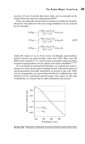
As an example for testing this technique, we evaluate the axial re-
sponse of a clear circular pupil imaging system, affected by spherical
and longitudinal chromatic aberrations as shown in Fig. 4.26. With-
out loss of generality we assume here that the SA coefficient has a flat
behavior for the considered spectral range. Once again, for the sake
of simplicity, we assume that no other aberrations are present.

400
Aberration coefficient (nm) –200
200

0

δW
–400 W 40 20

400 500 600 700
Wavelength: λ (nm)

FIGURE 4.26 Aberration coefficients associated with the system under issue.