Page 169 - Phase Space Optics Fundamentals and Applications

150 Chapter Four

We consider 36 axial positions characterized by defocus coefficient
values in a uniform sequence. We follow the same procedure as in
earlier sections for the digital calculation of the RWD RW q (x , ).
0,0
It is worth mentioning that for this pupil is possible to achieve an
analytical result for the monochromatic axial behavior of the system
for any value of W , W 40 , and , namely, 12

20
2
2

2
a 1 W ( ) + 2W 40 W ( )

20
20
I (z) = F √ − F √
2 f ( f + z) W 40 W 40 W 40
(4.96)
where
z
2
i t
F(z) = exp dt (4.97)
2
0
is the complex form of Fresnel integral. This analytical formula is used
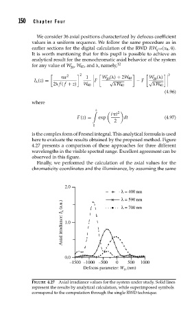
here to evaluate the results obtained by the proposed method. Figure
4.27 presents a comparison of these approaches for three different
wavelengths in the visible spectral range. Excellent agreement can be
observed in this figure.
Finally, we performed the calculation of the axial values for the
chromaticity coordinates and the illuminance, by assuming the same

2.0
λ = 400 nm
λ = 590 nm
Axial irradiance: I λ (a.u.) 1.0
λ = 700 nm

0.0
–1500 –1000 –500 0 500 1000
Defocus parameter: W (nm)
20

FIGURE 4.27 Axial irradiance values for the system under study. Solid lines
represent the results by analytical calculation, while superimposed symbols
correspond to the computation through the single RWD technique.