Page 166 - Phase Space Optics Fundamentals and Applications

The Radon-Wigner Transform 147

1.0 1.0
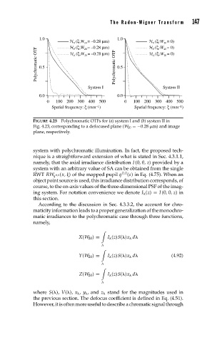
H X (ξ;W 20 = –0.28 μm) H X (ξ;W 20 = 0)
H Y (ξ;W 20 = 0)
H Y (ξ;W 20 = –0.28 μm)
Polychromatic OTF 0.5 H Z (ξ;W 20 = –0.28 μm) Polychromatic OTF 0.5 H Z (ξ;W 20 = 0)

System I System II
0.0 0.0
0 100 200 300 400 500 0 100 200 300 400 500
Spatial frequency: ξ (mm –1 ) Spatial frequency: ξ (mm –1 )

FIGURE 4.25 Polychromatic OTFs for (a) system I and (b) system II in
Fig. 4.23, corresponding to a defocused plane (W 20 =−0.28 m) and image
plane, respectively.

system with polychromatic illumination. In fact, the proposed tech-
nique is a straightforward extension of what is stated in Sec. 4.3.1.1,
namely, that the axial irradiance distribution I (0, 0,z) provided by a
system with an arbitrary value of SA can be obtained from the single
RWT RW q (x, ) of the mapped pupil q 0,0 (s) in Eq. (4.75). When an
0,0
object point source is used, this irradiance distribution corresponds, of
course, to the on-axis values of the three-dimensional PSF of the imag-
ing system. For notation convenience we denote I (z) = I (0, 0,z)in
this section.
According to the discussion in Sec. 4.3.3.2, the account for chro-
maticityinformationleadstoapropergeneralizationofthemonochro-
matic irradiances to the polychromatic case through three functions,
namely,

X(W 20 ) = I (z)S( )x d

Y(W 20 ) = I (z)S( )x d (4.92)

Z(W 20 ) = I (z)S( )x d

where S( ), V( ), x , y , and z stand for the magnitudes used in
the previous section. The defocus coefficient is defined in Eq. (4.51).
However, it is often more useful to describe a chromatic signal through