Page 165 - Phase Space Optics Fundamentals and Applications

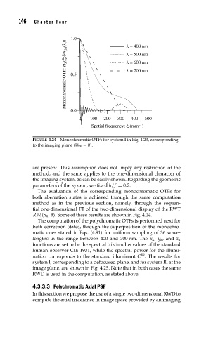
146 Chapter Four

1.0 λ = 400 nm
Monochromatic OTF: H λ (ξ;δW 20 (λ)) 0.5 λ = 600 nm

λ = 500 nm

λ = 700 nm

0.0
0 100 200 300 400 500
–1
Spatial frequency: ξ (mm )
FIGURE 4.24 Monochromatic OTFs for system I in Fig. 4.23, corresponding
to the imaging plane (W 20 = 0).

are present. This assumption does not imply any restriction of the
method, and the same applies to the one-dimensional character of
the imaging system, as can be easily shown. Regarding the geometric
parameters of the system, we fixed h/f = 0.2.
The evaluation of the corresponding monochromatic OTFs for
both aberration states is achieved through the same computation
method as in the previous section, namely, through the sequen-
tial one-dimensional FT of the two-dimensional display of the RWT
RW t (x , ). Some of these results are shown in Fig. 4.24.
The computation of the polychromatic OTFs is performed next for
both correction states, through the superposition of the monochro-
matic ones stated in Eqs. (4.91) for uniform sampling of 36 wave-
lengths in the range between 400 and 700 nm. The x , y , and z
functions are set to be the spectral tristimulus values of the standard
human observer CIE 1931, while the spectral power for the illumi-
49
nation corresponds to the standard illuminant C . The results for
system I, corresponding to a defocused plane, and for system II, at the
image plane, are shown in Fig. 4.25. Note that in both cases the same
RWD is used in the computation, as stated above.

4.3.3.3 Polychromatic Axial PSF
In this section we propose the use of a single two-dimensional RWD to
compute the axial irradiance in image space provided by an imaging