Page 346 - Phase Space Optics Fundamentals and Applications

Sampling and Phase Space 327

From our previous discussions the WDF of u T (x) may be defined
as

k
{u T (x)}(x, k) = {u(x)}(x, k) ∗ { T (x)}(x, k) (10.27)
and therefore the PSD for u T (x) is given by the convolution along k
of the PSD of u(x) and the PSD of the comb function shown in Fig.
10.3b. The result of convolving the signal’s PSD with these Dirac delta
lines is that we obtain multiple copies, in k, of the original signal PSD.
More accurately we obtain strips of the original WDF separated by the
sampling period, and we obtain multiple copies of these strips in k.It
is very important that the distance between the center of adjacent strip
copies in k (which from our earlier comb function analysis is equal to
1/T) be greater than or equal to b. When b = 1/T, we get the PSD
shown in Fig. 10.7b, where we can see that the replicas are just shy of
overlapping one another. This is the optimum sampling case known
as the Nyquist limit. The signal may be reconstructed by multiplying
U T (k)by Trect(Tk) defined in Eq. (10.17). From Fourier theory this is
equivalent to convolving u T (x) with sinc(x/T). All three equivalent
expressions for reconstruction are given below in terms of the spatial
representation, FT and WDF.

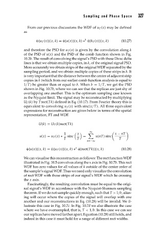
U(k) = U T (k)rect(Tk)
∞
1 , x − nT
x
u(x) = u T (x) ∗ sinc = u(nT) sinc
T T T
n=−∞
x
{u(x)}(x, k) = {u T (x)}(x, k) ∗ {rect(Tk)}(x, k) (10.28)
We can visualise this reconstruction as follows: The rect function WDF
illustrated in Fig. 10.5 convolves along the x axis in Fig. 10.7b. This rect
WDF has zero values for all values of k outside of the center order of
the sample’s signal WDF. Thus we need only visualize the convolution
of rect WDF with those strips of our signal’s WDF which lie crossing
the x axis.
Fascinatingly, the resulting convolution must be equal to the origi-
nal signal’s WDF in accordance with the Nyquist-Shannon sampling
theorem. If we do not sample quickly enough, such that T > 1/b, alias-
ing will occur where the copies of the signal will overlap with one
another and our reconstructions in Eq. (10.28) will be invalid. We il-
lustrate this case in Fig. 10.7c. In Fig. 10.7d we also illustrate the case
where we have oversampled, that is, T < 1/b. In this case we can see
our replicas have moved farther apart. Equation (10.28) still holds, and
indeed in this case it must hold for a range of different rect widths.