Page 350 - Phase Space Optics Fundamentals and Applications

Sampling and Phase Space 331

k k

x x

(a) (b)

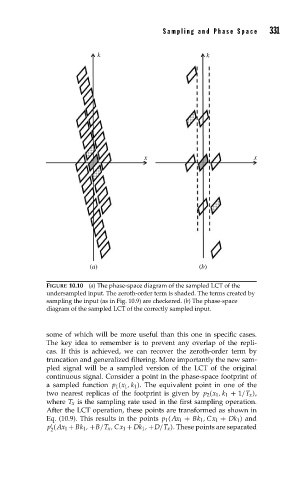
FIGURE 10.10 (a) The phase-space diagram of the sampled LCT of the
undersampled input. The zeroth-order term is shaded. The terms created by
sampling the input (as in Fig. 10.9) are checkered. (b) The phase-space
diagram of the sampled LCT of the correctly sampled input.

some of which will be more useful than this one in specific cases.
The key idea to remember is to prevent any overlap of the repli-
cas. If this is achieved, we can recover the zeroth-order term by
truncation and generalized filtering. More importantly the new sam-
pled signal will be a sampled version of the LCT of the original
continuous signal. Consider a point in the phase-space footprint of
a sampled function p 1 (x 1 ,k 1 ). The equivalent point in one of the
two nearest replicas of the footprint is given by p 2 (x 1 ,k 1 + 1/T x ),
where T x is the sampling rate used in the first sampling operation.
After the LCT operation, these points are transformed as shown in
Eq. (10.9). This results in the points p 1 (Ax 1 + Bk 1 ,Cx 1 + Dk 1 ) and
p (Ax 1 + Bk 1 , +B/T x ,Cx 1 + Dk 1 , +D/T x ). These points are separated

2