Page 348 - Phase Space Optics Fundamentals and Applications

Sampling and Phase Space 329

We note for the first time an interesting observation. Regardless
of what LCT caused phase space to be compact in some direction,
the sampling representation can always be based on the assumption
of a chirped signal. In addition, this does not change the number
of samples despite any bandwidth compression or expansion. From
Eq. (10.31) we can see that only two parameters of the LCT are em-
ployed in interpolation.

10.5 Simulating an Optical System:
Sampling at the Input and Output
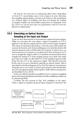
So far, we have discussed how to reconstruct a signal from its samples.
Often we encounter the case where a signal is sampled, an LCT is
applied to this discrete signal and the result of this is again sampled.
This arises in numerical simulations, where the input and output are
necessarily discrete, and when modeling paraxial optical systems with
discrete elements such as SLMs and CCD cameras. In this section, we
demonstrate how to sample a wave field which then undergoes a LCT,
how to sample the output of this LCT and then reconstruct from these
samples the analog LCT of the original analog wave field. Our major
goal here is to make sure that the LCT of the sampled signal actually
looks like the LCT of the continuous signal. This should obviously
be the case if we are to effectively simulate an optical system. This is
described by the block diagram in Fig. 10.8. We make two assumptions
about the input wave field: (1) It has approximately finite bandwidth,
and (2) it has approximately finite support. Both of these assumptions
are described by Eq. (10.23).
Inthecaseofthesesignalsitispossibletoderivearigoroussampling
theorythatcanbeinterpretedandderivedinthesimplestpossibleway
by employing PSDs.
Consider the first process in Fig. 10.8, sampling of the input.
When a signal is sampled, its phase-space diagram is altered by the

Analogue signal
bandwdth b Sampling Discrete signal LCT Analogue signal
extent d
(Input wavefield)

Reconstruction
filtering Sampling
Analogue signal Discrete signal
(Output wavefield)

FIGURE 10.8 Block diagram of the problem considered in this section.