Page 349 - Phase Space Optics Fundamentals and Applications

330 Chapter Ten

addition of periodic replicas, as illustrated by Fig. 10.7. When a sig-
nal is transformed by a LCT, its phase-space diagram undergoes an
area-preserving (affine) coordinate transformation, as illustrated in
Fig. 10.1. The case for a sampled signal (which is produced by the
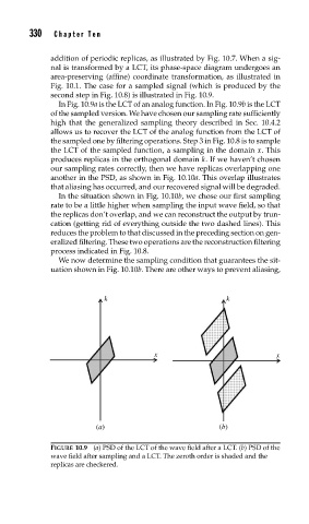
second step in Fig. 10.8) is illustrated in Fig. 10.9.
In Fig. 10.9a is the LCT of an analog function. In Fig. 10.9b is the LCT
of the sampled version. We have chosen our sampling rate sufficiently
high that the generalized sampling theory described in Sec. 10.4.2
allows us to recover the LCT of the analog function from the LCT of
the sampled one by filtering operations. Step 3 in Fig. 10.8 is to sample
the LCT of the sampled function, a sampling in the domain x. This
produces replicas in the orthogonal domain k. If we haven’t chosen
our sampling rates correctly, then we have replicas overlapping one
another in the PSD, as shown in Fig. 10.10a. This overlap illustrates
that aliasing has occurred, and our recovered signal will be degraded.
In the situation shown in Fig. 10.10b, we chose our first sampling
rate to be a little higher when sampling the input wave field, so that
the replicas don’t overlap, and we can reconstruct the output by trun-
cation (getting rid of everything outside the two dashed lines). This
reduces the problem to that discussed in the preceding section on gen-
eralized filtering. These two operations are the reconstruction filtering
process indicated in Fig. 10.8.
We now determine the sampling condition that guarantees the sit-
uation shown in Fig. 10.10b. There are other ways to prevent aliasing,

k k

x x

(a) (b)

FIGURE 10.9 (a) PSD of the LCT of the wave field after a LCT. (b) PSD of the
wave field after sampling and a LCT. The zeroth order is shaded and the
replicas are checkered.