Page 50 - Phase Space Optics Fundamentals and Applications

Wigner Distribution in Optics 31

From the latter equality we conclude that the value of the Wigner
distribution at some phase-space point (r, q) is related to the values
1
of all those pairs of points (r ± r , q ± q ) for which (r, q) is the

1
2 2
midpoint. Using, as we generally do, the analytic signal f (r) instead
1
of the real signal [ f (r) + f (r)] avoids the cross-terms that otherwise
∗
2
would automatically appear around q = 0.
The requirement of removing cross-terms without seriously affect-
ing the auto-terms has led to the Cohen class of bilinear signal rep-
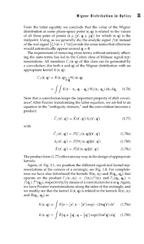
resentations. All members C f (r, q) of this class can be generated by
a convolution (for both r and q) of the Wigner distribution with an
appropriate kernel K(r, q):
C f (r, q) = K(r, q)∗ ∗W f (r, q)
r q

= K(r − r o , q − q ) W f (r o , q ) dr o dq (1.76)
o o o
Note that a convolution keeps the important property of shift covari-
ance! After Fourier transforming the latter equation, we are led to an
equation in the “ambiguity domain,” and the convolution becomes a
product:
¯
¯

C f (r , q ) = K(r , q )A f (r , q ) (1.77)

with
¯
C f (r , q ) = F[C f (r, q)](r , q ) (1.78a)

A f (r , q ) = F[W f (r, q)](r , q ) (1.78b)
¯

K(r , q ) = F[K(r, q)](r , q ) (1.78c)
The product form (1.77) offers an easy way in the design of appropriate
kernels.
Again, cf. Fig. 1.1, we position the different signal and kernel rep-
resentations at the corners of a rectangle, see Fig. 1.4. For complete-
ness we have also introduced the kernels R(r 1 , r 2 ) and ¯ R(q , q ) that
1 2
∗
operate on the product f (r 1 , r 2 ) = f (r 1 ) f (r 2 ) and ¯ f (q , q ) =
1
2
¯
f (q ) f (q ), respectively, by means of a convolution for r or q. Again,
¯ ∗
1 2
we have Fourier transformations along the sides of the rectangle, and
we readily see that the kernel K(r, q) is related to the kernels R(r 1 , r 2 )
and ¯ R(q , q )as
1 2

t
1
1
K(r, q) = R r + r , r − r exp(−i2 q r ) dr (1.79a)
2 2

1 1
t

K(r, q) = ¯ R q + q , q − q exp(i2 r q ) dq (1.79b)
2 2