Page 52 - Phase Space Optics Fundamentals and Applications

Wigner Distribution in Optics 33

Bilinear Signal Representation ¯ K(x ,u )

Wigner W(x, u), Eq. (1.14) 1
Pseudo-Wigner P(x, u; w), w( x )w (− x )
1
1
∗
2 2
Eq. (1.17)
Page exp(−i u |x |)

Kirkwood-Rihaczek exp(−i u x )

w-Rihaczek w(x ) exp(−i u x )

Levin cos( u x )
w-Levin w(x ) cos( u x )

Born-Jordan (sinc) sin( u x )/ u x

Zhao-Atlas-Marks (cone/ w(x ) | x | sin( u x )/ u x

windowed sinc)
2
Choi-Williams (exponential) exp[−(u x ) /
]
Generalized exponential exp[−(u /u o ) 2N ] exp[−(x /x o ) 2M ]

2

Spectrogram |S(x, u; w)| , A w (−x , −u )
Eq. (1.86)
¯
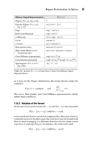
TABLE 1.2 Kernels K(x ,u ) of Some Basic Cohen-Class Bilinear Signal

Representations
as it does for the Wigner distribution, the kernel should satisfy the
condition
¯
∂K
¯
K(0,u ) = constant and = 0

∂x
x =0

The Levin, Born-Jordan, and Choi-Williams representations clearly
satisfy these conditions.
1.8.3 Rotation of the Kernel
In the case of two point sources (x − x 1 ) and (x − x 2 ), the cross-term
1
2 x − (x 1 + x 2 ) cos[2 (x 1 − x 2 )u]
2
was located such that we needed averaging in the u direction when we
wanted to remove it. In other cases, the cross-term may be located such
that we need averaging in a different direction; for two plane waves
exp(i2 u 1 x) and exp(i2 u 2 x), for instance, the cross-term reads
1
2 u − (u 1 + u 2 ) cos[2 (u 1 − u 2 )x]
2