Page 51 - Phase Space Optics Fundamentals and Applications

32 Chapter One

R(r + r, r − r ) ∗ Γ f (r + r, r − r )
1
1
1
1
2
2
r 2 2
C f (r, q)= K(r, q) ∗ ∗W f (r, q) C f (r , q )= K(r, q ) A f (r , q )
−
−

r q
−
R(q + q , q − q ) ∗ Γ f (q + q , q − q )
−
1
1
1
1
2 2 q 2 2
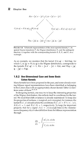
FIGURE 1.4 Schematic representation of the cross-spectral density , its
spatial Fourier transform ¯ , the Wigner distribution W, and the ambiguity
¯
function A, together with the corresponding kernels R, ¯ R, K, and K,ona
rectangle.
As an example, we mention that the kernel K(r, q) = (r) (q), for
which C f (r, q) = W f (r, q) is the Wigner distribution, corresponds to
¯
1
1
1

the kernels K(r , q ) = 1, R(r + r, r − r) = (r), and ¯ R(q + q ,

2
2
2
1

q − q ) = (q).
2
1.8.2 One-Dimensional Case and Some Basic
Cohen Kernels
Many kernels have been proposed in the past, and some already exist-
ing bilinear signal representations have been identified as belonging
to the Cohen class with an appropriately chosen kernel. Table 1.2 men-
tions some of them. 30,31,36
In designing kernels, one may try to keep the interesting properties
of the Wigner distribution; this reflects itself in conditions for the ker-
nel. We recall that shift covariance is already maintained. To keep also
the properties of realness, x marginal, and u marginal, for instance, the
¯
¯
kernel K(x ,u ) shouldsatisfytheconditions K(x ,u ) = K (−x , −u ),

¯ ∗

¯
¯

K(0,u ) = 1, and K(x , 0) = 1, respectively. To keep the important
property that for a signal f (x) =| f (x)| exp[i2 (x)] the instanta-
neous frequency d /dx should follow from the bilinear representation
through

uC f (x, u) du
d
=
dx
C f (x, u) du