Page 57 - Phase Space Optics Fundamentals and Applications

38 Chapter One

/2 0
According to Eq. (1.85), and using the fact that xx − > 0, we get
xx
o = 41 . The second-order moment in this direction, 41 ◦ = 0.057, is
◦
xx
smaller than in any other direction, while the second-order moment
in the orthogonal direction, −49 ◦ = 2.01, is the largest. The fractional
xx
1
Fourier transform F (x) of the signal f (x) for the angle = o − =
2
◦
−49 can now be calculated by using a discrete fractional Fourier
transformation algorithm. The next step is to calculate the windowed
(x, u; w) ofthefractionalFouriertransform F (x)
Fouriertransform S F
and to use it in Eq. (1.89).
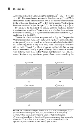
The results of this analysis are presented in Fig. 1.6. The pseudo-
Wignerdistribution P f (x, u; w) isshowninFig.1.6a.Thesmoothedin-
terferogram P f (x, u; w, z), calculated by the standard definition (1.88),
i.e., combining terms along the u axis, with a rectangular window
z(t) = rect(t/T) and T = 15, is presented in Fig. 1.6b. We see that
some cross-terms already appear, although the auto-terms are still
very different from those in the Wigner distribution in Fig. 1.6a. The
reason lies in the very significant spread of one component along the

P f (x,u;w) P f (x,u;w,z)
x x

u u
(a) (b)
γ γ
P f (x,u;w,z) P f (x,u;w,z)
x x

u u
(c) (d)

FIGURE 1.6 (a) Pseudo-Wigner distribution P f (x, u; w) of the signal f (x);
(b) smoothed interferogram P f (x, u; w, z) calculated in the frequency
domain, with a rectangular window z;(c) smoothed interferogram

P (x, u; w, z) calculated in the optimal frequency domain, with a rectangular
f

window z;(d) smoothed interferogram P (x, u; w, z) calculated in the
f
optimal frequency domain, with a Hann(ing) window z.