Page 65 - Phase-Locked Loops Design, Simulation, and Applications

MIXED-SIGNAL PLL ANALYSIS Ronald E. Best 46

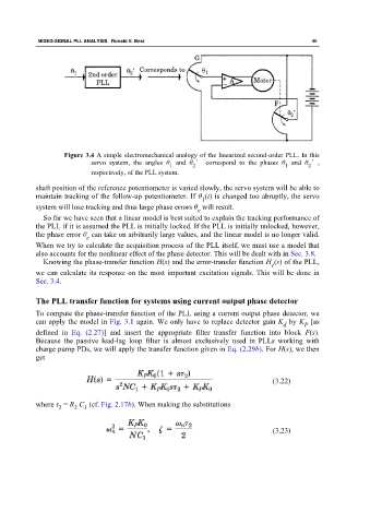
Figure 3.4 A simple electromechanical analogy of the linearized second-order PLL. In this
servo system, the angles θ and θ ′ correspond to the phases θ and θ ′,
1
2
2
1
respectively, of the PLL system.
shaft position of the reference potentiometer is varied slowly, the servo system will be able to
maintain tracking of the follow-up potentiometer. If θ (t) is changed too abruptly, the servo
1
system will lose tracking and thus large phase errors θ will result.
e
So far we have seen that a linear model is best suited to explain the tracking performance of
the PLL if it is assumed the PLL is initially locked. If the PLL is initially unlocked, however,
the phase error θ can take on arbitrarily large values, and the linear model is no longer valid.
e
When we try to calculate the acquisition process of the PLL itself, we must use a model that
also accounts for the nonlinear effect of the phase detector. This will be dealt with in Sec. 3.8.
Knowing the phase-transfer function H(s) and the error-transfer function H (s) of the PLL,
e
we can calculate its response on the most important excitation signals. This will be done in
Sec. 3.4.

The PLL transfer function for systems using current output phase detector
To compute the phase-transfer function of the PLL using a current output phase detector, we
can apply the model in Fig. 3.1 again. We only have to replace detector gain K by K [as
d P
defined in Eq. (2.27)] and insert the appropriate filter transfer function into block F(s).
Because the passive lead-lag loop filter is almost exclusively used in PLLs working with
charge pump PDs, we will apply the transfer function given in Eq. (2.29b). For H(s), we then
get

(3.22)

where τ = R C (cf. Fig. 2.17b). When making the substitutions
2 2 1

(3.23)