Page 70 - Phase-Locked Loops Design, Simulation, and Applications

MIXED-SIGNAL PLL ANALYSIS Ronald E. Best 49

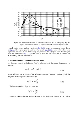
Figure 3.6 The transient response of a linear second-order PLL to a frequency step Δω
1
applied to its reference input at t = 0. (Adapted from Gardner with permission.)
Applying the inverse Laplace transform to Eq. (3.33), we get the phase error curves shown
in Fig. 3.6. If we again apply the final value theorem to Eq. (3.29), it turns out the phase error
approaches 0 when t → ∞. This is only true, however, for high-gain loops. For low-gain
loops, the numerator of Eq. (3.33) would have an additional first-order term in s; hence, the
phase error θ (∞) becomes nonzero.
e

Frequency ramp applied to the reference input

If a frequency ramp is applied to the PLL’s reference input, the angular frequency ω is
1
given by

(3.34)

where is the rate of change of the reference frequency . Because the phase θ (t) is the
1
integral over the frequency variation, we get

(3.35)

The Laplace transform Θ (s) now becomes
1

(3.36)

Assuming a high-gain loop again and applying the final value theorem of the Laplace