Page 73 - Phase-Locked Loops Design, Simulation, and Applications

MIXED-SIGNAL PLL ANALYSIS Ronald E. Best 51
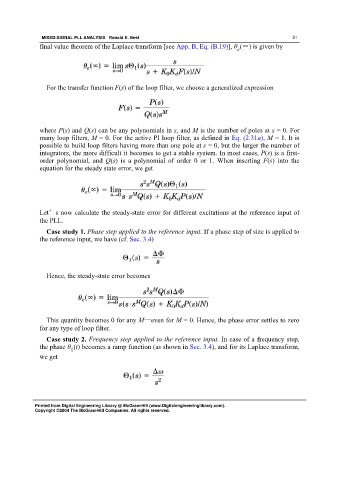
final value theorem of the Laplace transform [see App. B, Eq. (B.19)], θ (∞) is given by
e

For the transfer function F(s) of the loop filter, we choose a generalized expression

where P(s) and Q(s) can be any polynomials in s, and M is the number of poles at s = 0. For
many loop filters, M = 0. For the active PI loop filter, as defined in Eq. (2.31a), M = 1. It is
possible to build loop filters having more than one pole at s = 0, but the larger the number of
integrators, the more difficult it becomes to get a stable system. In most cases, P(s) is a first-
order polynomial, and Q(s) is a polynomial of order 0 or 1. When inserting F(s) into the
equation for the steady state error, we get

Let’s now calculate the steady-state error for different excitations at the reference input of
the PLL.
Case study 1. Phase step applied to the reference input. If a phase step of size is applied to
the reference input, we have (cf. Sec. 3.4)

Hence, the steady-state error becomes

This quantity becomes 0 for any M—even for M = 0. Hence, the phase error settles to zero
for any type of loop filter.

Case study 2. Frequency step applied to the reference input. In case of a frequency step,
the phase θ (t) becomes a ramp function (as shown in Sec. 3.4), and for its Laplace transform,
1
we get

Printed from Digital Engineering Library @ McGraw-Hill (www.Digitalengineeringlibrary.com).
Copyright ©2004 The McGraw-Hill Companies. All rights reserved.