Page 193 - Photodetection and Measurement - Maximizing Performance in Optical Systems

Stability and Tempco Issues

186 Chapter Eight

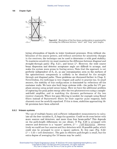
L ij
S 1 D 1

a

S 2 D 2
Figure 8.21 Resolution of the four-beam configuration is maximized by
increasing the difference between “short” and “long” path lengths.

tering attenuation of liquids in water treatment processes. Even without sta-
bilization of the source powers, and without correction for sensitivity changes
in the receivers, the technique can be used to determine a with good stability.
To maximize sensitivity we must maximize the difference between diagonal and
straight-through paths (Fig. 8.21), and hence L*. However, the wide source
beam dispersion and detector acceptance angle are difficult to arrange, and
make the system more prone to fouling errors. Note that the approach is not
perfectly independent of S i, D j, as any contamination seen on the surfaces of
the optoelectronic components is unlikely to be identical for the straight
through and diagonal paths. These problems are discussed further in Chap. 9.
Nevertheless, the technique is very elegant and useful in practice too. In small
sensors, the stability of this configuration is dominated by reflections off the
container walls. We have also built large systems with ª1m paths for UV gas-
phase sensing using pulsed xenon lamps. Here we have the additional problem
of capturing the peak pulse energy after the two photoreceivers using a sample-
and-hold amplifier, and in matching the dynamic performance of the two
receiver channels. Where low-pass filtering is needed, for example using Bessel
filters instead of Butterworth filters for their superior pulse response, both
channels must be carefully equalized. If this is done, stabilities approaching 16-
bit precision have been achieved.

8.6.2 N-beam systems
The use of multiple beams and sufficient independent measurements to calcu-
late all the free variables S i , D j begs the question: Could we do even better with
more sources and detectors, and more than four beam-paths? This depends
on the path-length differences we can obtain. If Fig. 8.20 is arranged with
sources and detectors in a “square” pattern, L* ª cell dimension . Alterna-
tively we could use four sources and four detectors with 16 possible paths, which
could also be arranged to cover a square pattern. In this case (Fig. 8.22)
L* ª 1.53 ¥ (cell dimension). The gain in effective path-length is small, but the
extra degree of averaging the 16 beams may be useful.

Downloaded from Digital Engineering Library @ McGraw-Hill (www.digitalengineeringlibrary.com)
Copyright © 2004 The McGraw-Hill Companies. All rights reserved.
Any use is subject to the Terms of Use as given at the website.