Page 350 - Physical Principles of Sedimentary Basin Analysis

332 Gravity and gravity anomalies

x

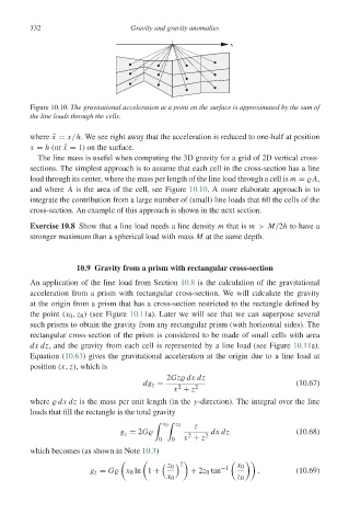
Figure 10.10. The gravitational acceleration at a point on the surface is approximated by the sum of
the line loads through the cells.

x
where ˆ = x/h. We see right away that the acceleration is reduced to one-half at position
x
x = h (or ˆ = 1) on the surface.
The line mass is useful when computing the 3D gravity for a grid of 2D vertical cross-
sections. The simplest approach is to assume that each cell in the cross-section has a line
load through its center, where the mass per length of the line load through a cell is m = A,
and where A is the area of the cell, see Figure 10.10. A more elaborate approach is to
integrate the contribution from a large number of (small) line loads that fill the cells of the
cross-section. An example of this approach is shown in the next section.

Exercise 10.8 Show that a line load needs a line density m that is m > M/2h to have a
stronger maximum than a spherical load with mass M at the same depth.

10.9 Gravity from a prism with rectangular cross-section
An application of the line load from Section 10.8 is the calculation of the gravitational
acceleration from a prism with rectangular cross-section. We will calculate the gravity
at the origin from a prism that has a cross-section restricted to the rectangle defined by
the point (x 0 , z 0 ) (see Figure 10.11a). Later we will see that we can superpose several
such prisms to obtain the gravity from any rectangular prism (with horizontal sides). The
rectangular cross-section of the prism is considered to be made of small cells with area
dx dz, and the gravity from each cell is represented by a line load (see Figure 10.11a).
Equation (10.63) gives the gravitational acceleration at the origin due to a line load at
position (x, z), which is
2Gz dx dz
dg z = (10.67)
2
x + z 2
where dx dz is the mass per unit length (in the y-direction). The integral over the line
loads that fill the rectangle is the total gravity

x 0 z 0 z
g z = 2G 2 2 dx dz (10.68)
0 0 x + z
which becomes (as shown in Note 10.3)

2
z 0 −1 x 0
g z = G x 0 ln 1 + + 2z 0 tan . (10.69)
x 0 z 0