Page 353 - Physical Principles of Sedimentary Basin Analysis

10.10 Gravity from a 2D polygonal body 335

50
1
3
40
2
dg [mGal] 20
30

10

0
0 2 4 6 8 10
distance [km]
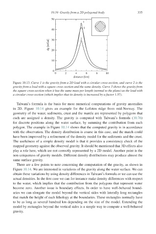
Figure 10.13. Curve 1 is the gravity from a 2D load with a circular cross-section, and curve 2 is the
gravity from a load with a square cross-section and the same density. Curve 3 shows the gravity from
the square cross-section when it has the same mass per length (normal to the plane) as the load with
a circular cross-section (which implies that its density is increased by a factor 1.57).

Talwani’s formula is the basis for most numerical computations of gravity anomalies
in 2D. Figure 10.14 gives an example for the Lofoten ridge from mid-Norway. The
geometry of the water, sediments, crust and the mantle are represented by polygons that
each are assigned a density. The gravity is computed with Talwani’s formula (10.76)
for discrete positions along the water surface, by summing the contribution from each
polygon. The example in Figure 10.14 shows that the computed gravity is in accordance
with the observation. The density distribution is coarse in this case, and the match could
have been improved by a refinement of the density model for the sediments and the crust.
The usefulness of a simple density model is that it provides a consistency check of the
mapped geometry against the observed gravity. It should be mentioned that 3D effects also
play a role here, which are not correctly represented by a 2D model. Another point is the
non-uniqueness of gravity models. Different density distributions may produce almost the
same surface gravity.
There are a few points to note concerning the computation of the gravity, as shown in
Figure 10.14. We are interested in variations of the gravity along the water surface. We can
obtain these variations by using density differences in Talwani’s formula or we can use the
actual densities. In the first case we can for instance make density differences with respect
to the water, which implies that the contribution from the polygons that represent water
become zero. Another issue is boundary effects. In order to have well-behaved bound-
aries we can elongate the model beyond the vertical sides with laterally long rectangles
that match the height of each lithology at the boundaries. These rectangles normally have
to be as long as several hundred km depending on the size of the model. Extending the
model by rectangles beyond the vertical sides is a simple way to compute a well-behaved
gravity.