Page 382 - Physical Chemistry

lev38627_ch12.qxd 3/18/08 2:41 PM Page 363

363
From (12.35) we have Section 12.6
Two-Component
l
x v B x P* B ideal soln. (12.36) Liquid–Vapor Equilibrium
B

l
x C v x P* C
C
Let B be the more volatile component, meaning that P* P*. Equation (12.36) then
C
B
l
v
l
v
shows that x /x x /x . The vapor above an ideal solution is richer than the liquid
C
C
B
B
in the more volatile component (Fig. 9.18b). Equations (12.35) and (12.36) apply at
any pressure where liquid–vapor equilibrium exists, not just at point D.
Now let us isothermally lower the pressure below point D, causing more liquid to
vaporize. Eventually, we reach point F in Fig. 12.8b, where the last drop of liquid
vaporizes. Below F, we have only vapor. For any point on the line between D and F,
liquid and vapor phases coexist in equilibrium.
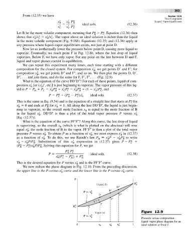
We can repeat this experiment many times, each time starting with a different
composition for the closed system. For composition x
, we get points D
and F
; for
B
composition x , we get points D and F ; and so on. We then plot the points D, D
,
B
D , . . . and join them, and do the same for F, F
, F , . . . (Fig. 12.9).
What is the equation of the curve DD
D ? For each of these points, liquid of com-
l
l
position x [or (x )
, etc.] is just beginning to vaporize. The vapor pressure of this liq-
B
B
l
l
l
l
uid is P P P x P* x P* x P* (1 x )P*, and
C
C
B B
B
B B
C C
B
l
P P* 1P* P*2x ideal soln. (12.37)
C B C B
This is the same as Eq. (9.54) and is the equation of a straight line that starts at P* for
C
l
l
x 0 and ends at P* for x 1. All along the line DD
D , the liquid is just begin-
B B B
ning to vaporize, so the overall mole fraction x is equal to the mole fraction of B
B
l
in the liquid x . DD
D is thus a plot of the total vapor pressure P versus x l
B B
[Eq. (12.37)].
What is the equation of the curve FF
F ? Along this curve, the last drop of liquid
is vaporizing, so the overall x (which is what is plotted on the abscissa) will now
B
v
equal x , the mole fraction of B in the vapor. FF
F is then a plot of the total vapor
B
v
v
l
pressure P versus x . To obtain P as a function of x , we must express x in (12.37)
B
B
B
v
v
l
as a function of x . To do this, we use Raoult’s law P x P x P* to write
B
B
B
B
B
v
l
x x P/P*. Substitution of this x l expression in (12.37) gives P P*
B B B B C
v
(P* P*)x P/P*. Solving this equation for P, we get
B C B B
P* P*
P B C ideal soln. (12.38)
v
x 1P* P*2 P*
B
B
B
C
v
This is the desired equation for P versus x and is the FF
F curve.
B
We now redraw the phase diagram in Fig. 12.10. From the preceding discussion,
v
l
the upper line is the P-versus-x curve and the lower line is the P-versus-x curve.
B B
P
*
Liquid (l) P B
D′′
P vs. x l D′
B
D F′′
l F′
F
P * C
Vapor ( ) Figure 12.9
y
P vs. x
B
Pressure-versus-composition
liquid–vapor phase diagram for an
0 x B x′ B x′′ B 1 ideal solution at fixed T.