Page 386 - Physical Chemistry

lev38627_ch12.qxd 3/18/08 2:41 PM Page 367

367
Ideal Solution at Fixed Pressure Section 12.6
Now consider the fixed-pressure liquid–vapor phase diagram of two liquids that form Two-Component
Liquid–Vapor Equilibrium
an ideal solution. The explanation is quite similar to the fixed-temperature case just
discussed in great and somewhat repetitious detail, so we can be brief here. We plot
T versus x , the overall mole fraction of one component. The phase diagram is
B
Fig. 12.12.
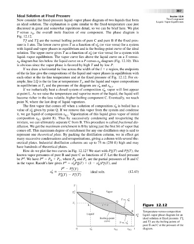
T * and T * are the normal boiling points of pure C and pure B if the fixed pres-
C B
l
sure is 1 atm. The lower curve gives T as a function of x (or vice versa) for a system
B
with liquid and vapor phases in equilibrium and is the boiling-point curve of the ideal
v
solution. The upper curve gives T as a function of x (or vice versa) for a system with
B
liquid–vapor equilibrium. The vapor curve lies above the liquid curve on a T-versus-
x diagram but lies below the liquid curve on a P-versus-x diagram (Fig. 12.10). This
B B
is obvious since the vapor phase is favored by high T and by low P.
If we draw a horizontal tie line across the width of the l v region, the endpoints
of the tie line give the compositions of the liquid and vapor phases in equilibrium with
each other at the tie-line temperature and at the fixed pressure of Fig. 12.12. For ex-
ample, line LQ is the tie line at temperature T , and the liquid and vapor compositions
1
in equilibrium at T and the pressure of the diagram are x
and x .
1 B B,1
If we isobarically heat a closed system of composition x
, vapor will first appear
B
at point L. As we raise the temperature and vaporize more of the liquid, the liquid will
become richer in the less volatile, higher-boiling component C. Eventually, we reach
point N, where the last drop of liquid vaporizes.
The first vapor that comes off when a solution of composition x
is boiled has a
B
v
value of x given by point Q. If we remove this vapor from the system and condense
B
it, we get liquid of composition x . Vaporization of this liquid gives vapor of initial
B,1
composition x (point R). Thus by successively condensing and revaporizing the
B,2
mixture, we can ultimately separate C from B. This procedure is called fractional dis-
tillation. We get the maximum enrichment in B by taking just the first bit of vapor that
comes off. This maximum degree of enrichment for any one distillation step is said to
represent one theoretical plate. By packing the distillation column, we in effect get
many successive condensations and revaporizations, giving a column with several the-
oretical plates. Industrial distillation columns are up to 75 m (250 ft) high and may
have hundreds of theoretical plates.
How do we plot the two curves in Fig. 12.12? We start with P*(T) and P*(T), the
B C
known vapor pressures of pure B and pure C as functions of T. Let the fixed pressure
#
#
be P . We have P P P , where P and P are the partial pressures of B and C
B C B C
l
#
l
in the vapor. Raoult’s law gives P x P*(T) (1 x )P*(T), and
B B B C
#
P P*1T2
C
x ideal soln. (12.43)
l
B
P*1T2 P*1T2
C
B
T
T * N Vapor
C

T vs. x
Q B
T 1
L l Figure 12.12
R Temperature-versus-composition
Liquid T * liquid–vapor phase diagram for an
Boiling-point B ideal solution at fixed pressure. T* B
curve l and T* are the boiling points of
T vs. x C
B
pure B and C at the pressure of the
0 x B ′ x B,1 x B,2 1 diagram.