Page 117 - Practical Control Engineering a Guide for Engineers, Managers, and Practitioners

92 Chapter Four

of the controlled system was shown to be described by the two trans-
fer functions, one for the process GP and one for the controller Gc. The
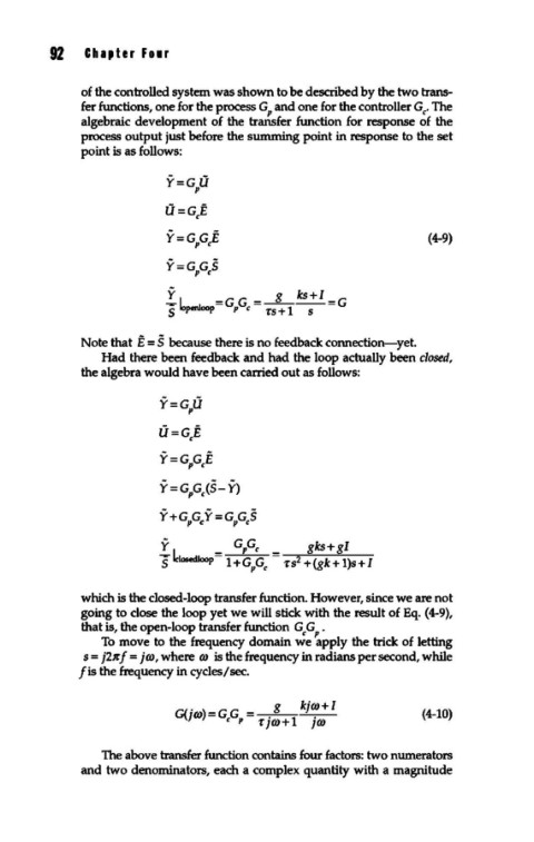
algebraic development of the transfer function for response of the
process output just before the summing point in response to the set
point is as follows:

Y=GpGcE (4-9)
Y=GpGcS

Y g ks+I
S~oop=GpGc= -rs+1-s-=G

Note that E = S because there is no feedback connection-yet.
Had there been feedback and had the loop actually been closed,
the algebra would have been carried out as follows:

U=GE
c
Y=G,GCE

Y = GpGc(S- Y)

Y + GpGc Y = GpGcS
y _ G,Gc gks+gl
S lc~osedloop- 1 + G G -rs +(gk+ 1)s+ I
2
p c
which is the closed-loop transfer function. However, since we are not
going to close the loop yet we will stick with the result of Eq. (4-9),
that is, the open-loop transfer function GcG .
To move to the frequency domain we ~pply the trick of letting
s = j2tc f = jro, where ro is the frequency in radians per second, while
fis the frequency in cycles/sec.

G( "ro)=G G =-g_kjro+l (4-10)
I c P -r jro+ 1 jro

The above transfer function contains four factors: two numerators
and two denominators, each a complex quantity with a magnitude