Page 119 - Practical Control Engineering a Guide for Engineers, Managers, and Practitioners

94 Chapter Four

c.:;~ 2
~
0 1.5
:=
e!
QJ t
"'tS
:5 0.5
}
<
oto-J to-1 tOO
-80

c.:;~ -100
~ -200
QJ
~ -t40
..c
ll.. -160
-180
to-J to-2 to-1 tOO
Frequency (/min)

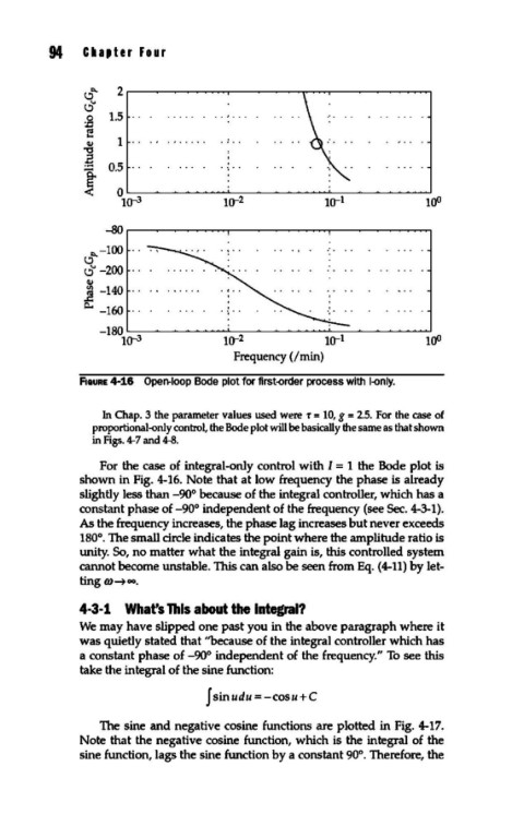
F1aURE 4-1.6 Open-loop Bode plot for first-order process with 1-only.

In Chap. 3 the parameter values used were T = 10, g = 2.5. For the case of
proportional-only control, the Bode plot will be basically the same as that shown
in Figs. 4-7 and 4-8.

For the case of integral-only control with I = t the Bode plot is
shown in Fig. 4-t6. Note that at low frequency the phase is already
slightly less than -90° because of the integral controller, which has a
constant phase of -90° independent of the frequency (see Sec. 4-3-t).
As the frequency increases, the phase lag increases but never exceeds
t80°. The small circle indicates the point where the amplitude ratio is
unity. So, no matter what the integral gain is, this controlled system
cannot become unstable. This can also be seen from Eq. (4-11) by let-
ting (.()~oo.
4-3-1 What's This about the Integral?
We may have slipped one past you in the above paragraph where it
was quietly stated that ''because of the integral controller which has
a constant phase of -90° independent of the frequency." To see this
take the integral of the sine function:

J sinudu =-cosu+C
The sine and negative cosine functions are plotted in Fig. 4-t7.
Note that the negative cosine function, which is the integral of the
sine function, lags the sine function by a constant 90°. Therefore, the