Page 120 - Practical Control Engineering a Guide for Engineers, Managers, and Practitioners

A New Domain and More Process Models 95

1rJ~~~:-~~~~~~~~~~
0.8
0.6
0.4

~ 0.2
.a
;a_ 0
~ -0.2
-0.4
-0.6
-0.8

Tune

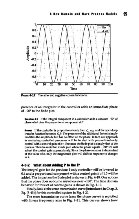
F1auRE 4-17 The sine and negative cosine functions.

presence of an integrator in the controller adds an immediate phase
of -90° to the Bode plot.

Question 4-6 If the integral component in a controller adds a constant -90° of
phase what does the proportional component do?

Answer If the controller is proportional-only then Gc = k and the open-loop
transfer function becomes G k. The presence of the additional factor k simply
modifies the amplitude but has no effect on the phase. In fact, our approach
in analyzing controlled processes will be to start with proportional-only
control with a control gain of k = 1 because the Bode plot is simply that of the
process. Then to avoid too much gain when the phase equals -180° we will
adjust the control gain appropriately. Since the phase remains independent
of the value of k, only the magnitude plot will shift in response to changes
ink.

4-3-2 What about Adding P to the I?
The integral gain for the previous 1-only controller will be lowered to
0.4 and a proportional component with a control gain k of 1.0 will be
added. The impact on the Bode plot is shown in Fig. 4-18. One notices
that the phase does not come anywhere near -180°. The time domain
behavior for this set of control gains is shown in Fig. 4-19.
Finally, look at the error transmission curve [introduced in Chap. 3,
Eq. (3-43)] for this controlled system in Fig. 4-20.
The error transmission curve (sans the phase curve) is replotted
with linear frequency axes in Fig. 4-21. This curves shows how