Page 176 - Practical Control Engineering a Guide for Engineers, Managers, and Practitioners

An Underda01ped Process 151

tO ..... .
0
~
.a -tO
"t;! -20 o • I • • I I._,., J • • • • • I ol '•
6b
II.
~ -30 ... •'. '' .•.
-40to-3 to- 2 tOO to2

OF=~~--~~~~ .. ~.
.... ~~~ ~~
-50
(U
.! -tOO .. •,,•,•: ....... ,••
p.. ol
0
0
-t50 .... , .......... .
-200~~~----~~~--~~~~~~~~~~
to-3 to- 2 to- 1 tOO t0 1 to2
Frequency (Hz)

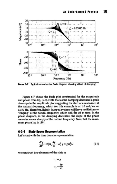
F1cauRE 8-7 Typical second-order Bode diagram showing effect of damping.

Figure 6-7 shows the Bode plot constructed for the magnitude
and phase from Eq. (6-6). Note that as the damping decreases a peak
develops in the amplitude plot suggesting the start of a resonance at
the natural frequency, which for this example is at 1.0 rad/ sec or
O.t59 Hz. Therefore, lightly damped systems will have oscillations or
"ringing" at the natural frequency which will die off in time. In the
phase diagram, as the damping decreases, the slope of the phase
curve increases sharply at the natural frequency. Note that the maxi-
mum phase lag is t80°.

6-2-4 State-Space Representation
Let's start with the time domain representation:

(6-7)

we construct two elements of the state as