Page 177 - Practical Control Engineering a Guide for Engineers, Managers, and Practitioners

152 Chapter Six

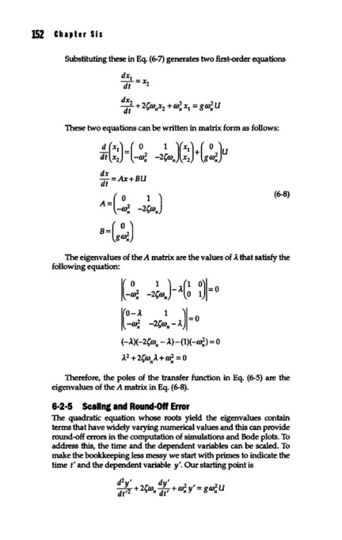
Substituting these in Eq. (6-7) generates two first-order equations
dx 1
dt=x2
dx2 2 _ 2
Tt + 2{conx2 +con x1 - gco,. u

These two equations can be written in matrix form as follows:

(6-8)
A-( 0 1 )
- -co; -2{con

The eigenvalues of the A matrix are the values of A. that satisfy the
following equation:

0 1 ) ;t(1 0)1-0
I( -co; -2{co,. - 0 1 -

I(~ -~.-!JI=O

(-A.)(-2{co,- A.)-(1)(-co;) = 0

Jt2 + 2{co,.A.+to; = 0
Therefore, the poles of the transfer function in Eq. (6-5) are the
eigenvalues of the A matrix in Eq. ( 6-8).
6·2·5 Scaling and Round-Off Error
The quadratic equation whose roots yield the eigenvalues contain
terms that have widely varying numerical values and this can provide
round-off errors in the computation of simulations and Bode plots. To
address this, the time and the dependent variables can be scaled. To
make the bookkeeping less messy we start with primes to indicate the
time t' and the dependent variable y'. Our starting point is

d2yl dy' 2 I - 2
dt'2 + 2{con tit'+ cony - gco, u