Page 344 - Practical Design Ships and Floating Structures

319

ST1.5 (S-line) inspecting its curvature, the crossing waterlines WL06, WLOI, and WLlO (S-lines) will
be automatically changed by the update operation on ST15. Then, the change of the three waterlines
causes a re-update of the buttock line and the gray station lines (R-lines). This automation of the cross
fairing enables designers to manipulate the wireframe model more efficiently by inspecting the global
curvature.

- SUM
-
R-Une

Figure 3: Example of the association based cross faring showing that all lines related to the changed
station line STl5 are updated automatically

4 GENERATION OF SURFACE MODEL FOR NON-MANIFOLD DATA STRUCTURE

4.1 Process of Surface Model Generation
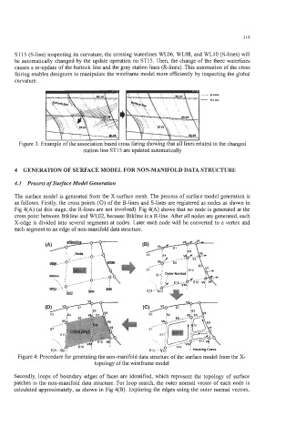
The surface model is generated from the X-surface mesh. The process of surface model generation is
as follows. Firstly, the cross points (0) of the B-lines and S-lines are registered as nodes as shown in
Fig 4(A) (at this stage, the R-lines are not involved). Fig 4(A) shows that no node is generated at the
cross point between Btkline and WL02, because Btkline is a R-line. After all nodes are generated, each
X-edge is divided into several segments at nodes. Later each node will be converted to a vertex and
each segment to an edge of non-manifold data structure.

Figure 4: Procedure for generating the non-manifold data structure of the surface model from the X-
topology of the wireframe model

Secondly, loops of boundary edges of faces are identified, which represent the topology of surface
patches in the non-manifold data structure. For loop search, the outer normal vector of each node is
calculated approximately, as shown in Fig 4(B). Exploring the edges using the outer normal vectors,