Page 357 - Practical Design Ships and Floating Structures

332

of analyses, the least squares method to obtain an approximate mathematical expression of the
response, and the nonlinear optimization method to determine the optimal design, Le., the minimum or
maximum response.
In this paper, as an example of the application of RSM to ship structural design, the optimization of the
transverse bulkhead structures of an oil tanker is performed. The results obtained and the know-how
accumulated in using this methodology for optimizing ship structural design are shown. Through the
research shown in this paper, the advantages of the RSM are clarified; i.e., the behavior of the solution
around the optimum is easily examined and the trade-off in the design can be carried out. Also, the
methodology is shown to be very powerful means of rationally reducing the number of structural
response analyses where efficiency of the analysis is very much expected.

2 RESPONSE SURFACE METHODOLOGY

2.1 Basic theories of RSM
A response surface is a curved surface that represents the relationship between the design variables x,
(i=l,. . ..,n) and the response y. This relationship can be presented by the following equation:
y=f(xl,..*-.,xn)+& (1)
where E is the random error in y. There is no restriction in the form of function fthat
approximates the response surface. However, for the sake of simplicity, a polynomial to express the
function f can be generally used. For example, if we use the second-order model with n design
variables, the model becomes:
n n n
Y = A 4- csixi + cc B,XiX, 4- E (2)
i=l 1st JW
To obtain the fonn of the above equation, it is necessary to determine the unknown parameter B.
For this purpose, we need a set of multiple design variables and the responses to those conditions (i.e.,
observations). To begin with, by replacing the second-order term (Le., xI2, xlx,, x22, etc.) with
x,,, =x,x2, etc., the equation is transformed to the first-order expression. Then, Eqn.2 can be
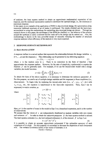
expressed, in matrix notation, as
y=x$+& (3)
where

B=

Here, pel is the number of terms in the model in Eqn.2 in a linearlized expression, and k is the number
of observations.
We assume that the values of E are independently distributed as random variables with zero means
and variances u2 . In order to obtain the unknown parameter p , the least squares method is utilized.
The least squares estimates (Le., the best unbiased estimates), b, of the element p in Eqn.3 are
b = (x‘x)-’xTy (4)
It is possible to obtain an accurate approximate polynomial if the estimation accuracy of each
component of b is high. For this purpose it is necessary to decrease the dispersion of each component
of b. The variance-covariance matrix of the vector of estimates, b, is
Vu@) = Vur(Cy)