Page 358 - Practical Design Ships and Floating Structures

333

= CVm(y)C7
Here C=(X'X)-'X'. Since Vm(y)=Vm(~)=a~I,then
Vm(b) = m2(XTX)-' (5)
It is understood from Eqn.5 that the variance-covariance matrix Vm(b) consists of the components
is
a2 and (X'X)-' . As mentioned above, a2 the variance of the random errors that are related to
the characteristics of the response y; thus it cannot be controlled. On the other hand (X'X)-' is
determined by the combination of the design variables. Therefore, the minimization of each
component of Vm(b) is possible if we minimize the dispersion of (X'X)-' . In this way, estimation
of at a high level of accuracy can be realized. This is the principle upon which the design of
experiment is based. Taking advantage of the advancement of recent computer technology, a few
numerical approaches of the design of experiment are proposed. In the design of experiment using a
Computer, a large number of candidate combinations of design variables are prepared beforehand, and
the minimum number of combinations are selected from them by using the optimum criterion. In this
paper, the D-optimal design, Khuri & Cornell (1 996), is used. The D-optimal design is a method that
determines a combination of design variables which maximizes the determinant of the matrix
M(= XT X / k) , which is called the moment matrix. In this method, by normalizing the coordinate of
the design variable between -1 to 1, D-efficiency ( DH ), which is the corrected value of the moment
matrix, is used as the criterion:
(Det[XTXP"
Def =
k
where p+l is the number of unknown parameters in Eqn.3.
Each (XrX)-' component decreases relatively if we choose the combination of the design variable
which maximizes the D@; therefore, accurate parameters for the polynomial equation can be
obtained.

2.2 Approximation of mpnse sdace wing p&nomal
In the actual design problems, the true solution may fluctuate or be discontinuous. In such cases, a
decrease of the search accuracy or failure of the search algorithm is often brought about if the
solution-search method uses the gradient of the response
surface. In response surface methodology, on the other I
hand, the least squares method using the polynomial as seen
in Eqn.2 is utilized and an alternative solution having a
smooth surface is obtained. The search efficiency of the
optimum solution is very good, since the optimization in the
alternative response surface finishes almost in a moment.
Moreover, this methodology has the advantage that it would P
be able to easily grasp the general property of the response z
by obtaining the approximate response surface which filters ;
the small discontinuity or fluctuations which are, in some
cases, inevitable (e.g., measuring errors in model
experiments, etc.). This advantage is very effective in the
initial design stage. If we consider the approximate
polynomial to be a Taylor series expansion of the solution, it
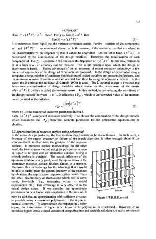
may be said that an approximation with sufficient accuracy Figure 1:T.B.H.D.model
is possible using a low-order polynomial if the region of
interest is narrow. To approximate the response in a wider
region, the introduction of higher order terms in the polynomial is considered. However, if we
introduce higher terms, a rapid increase of computing time and unstable solutions are easily anticipated.