Page 528 - Practical Design Ships and Floating Structures

503

Residual resistance coefficient CR can be predicted by the artificial neural networks presented in this
paper. The result is correlated against full-scale trials applying a resistance correlation coefficient CA,
which usually varies for different towing tanks. MAFUNTEK usually applies resistance correlation
coefficient values between -0.20 .1 O5 and -0.23 .lo" for conventional ships.
The roughness allowance ACF is calculated using hull surface roughness H in p (= 10" m). Typical
value of hull surface roughness is 150 p. Only positive values of AC,C are used.
AC, = [110.31.(H.V,)o.2' -403.33].Ci:v

3 DATABASE

Analyses are based on measurements performed in the towing tank at MAIUNTEK in recent two
decades. Special cases did not take part in analysis. The database includes 487 ships and 3481
measurement points. Analyses of the database are performed using Artificial Neural Networks Method.
A preliminary analysis of the database shows that higher accuracy can be achieved by using different
neural networks for different categories of ships.
Therefore one ship type or several similar ship types are grouped in one category. This allows using
different input parameters according to sensitivity analysis performed for each group. In addition pre-
weighting of input parameters can be tuned applying sensitivity analysis results. The pre-study led to
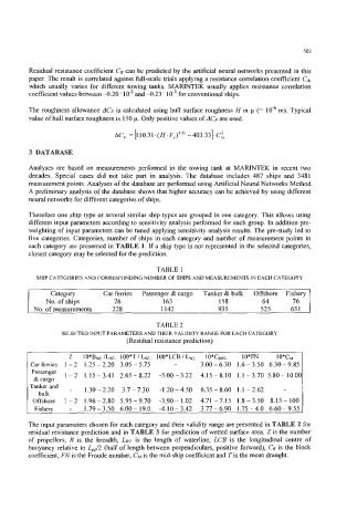
five categories. Categories, number of ships in each category and number of measurement points in
each category are presented in TABLE 1. If a ship type is not represented in the selected categories,
closest category may be selected for the prediction.
TABLE 1
SHIP CATEGORIES AND CORRESPONDMG NUMBER OF SHIPS AND MEASUREMENTS IN EACH CATEGORY
Category Car femes Passenger & cargo Tanker & bulk Offshore Fishery
No. of ships 26 163 158 64 76
No. of measurements 228 1 I42 935 525 65 1
TABLE 2
SELECTED INPUT PARAMETERS AND THEIR VALIDITY RANGE FOR EACH CATEGORY
(Residual resistance prediction)

Z IO*BN/Lw 100*TILw 100*LCB/Lw IO*CBw IO*FN IO*(&
Car ferries 1 - 2 1.25 - 2.20 3.05 - 5.75 3.00 - 6.30 1.6 - 3.50 6.30 - 9.85
Passenger 1-2 1.15-3.41 2.65-8.22 -5.00-3.22 4.15-8.10 1.1-3.70 5.80-10.00
& care0 -
Tankerand -
bulk 1.30-2.20 3.7-7.30 -1.20-4.50 6.35-8.60 1.1 -2.62
Offshore 1-2 1.96-2.80 5.95-9.70 -3.90-1.02 4.71-7.15 1.8-3.50 8.15-100
Fishery - 1.79-3.50 6.00-19.0 4.10-3.42 3.77-6.90 1.75-4.0 6.60-9.55
The input parameters chosen for each category and their validity range are presented in TABLE 2 for
residual resistance prediction and in TABLE 3 for prediction of wetted surface area Z is the number
of propellers, B is the breadth, LWL is the length of waterline, LCB is the longitudinal centre of
buoyancy relative to L,d2 (half of length between perpendiculars, positive forward), Cg is the block
coefficient, FN is the Froude number, CM is the mid-ship coefficient and Tis the mean draught.