Page 184 - Principles and Applications of NanoMEMS Physics

172 Chapter 4

induce a certain time evolution of a spin state by the fine perturbation that
varying the amplitude, frequency, and phase of the control Hamiltonian
affords.
The analysis of spin rotations is facilitated by describing the motion with
respect to the so-called rotating frame [193], [194]. This is a coordinate
system that rotates with respect to the z ˆ axis at a frequency ω . A given
RF
rot

state in the rotating frame ψ and the corresponding state ψ in the laboratory
(non-rotating) frame are related by [191],
ψ rot = exp ( ω−i tI ) ψ . (22)
RF z

It can be shown by substitution of (22) into Schödinger’s equation, that in
the rotating frame and in the presence of many, e.g., r, applied RF fields, the
system and control Hamiltonians adopt the forms [194],

j
H = = ¦ 2 πJ I i I , (23)
sys ij z z
i < j
and
i
r
t
t
I
H = ¦ −= ω r [cos ( ( ω r − ω i ) + φ r ) +sin ( ( ω r − ω i ) + φ I i
) ]. (24)
control 1 RF 0 x RF 0 y
r , i
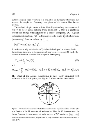
The effect of the control Hamiltonian is most easily visualized with
reference to the Bloch sphere, see Fig. 4-17, whose surface contains the
Qubit Tip
Qubit Tip
Trajectories
Trajectories

Figure 4-17. Bloch sphere surface: Dashed lines delineate the trajectories of the tip of a qubit
as a function of the RF pulse strength and duration. When the RF frequency equals the
°
Larmor frequency, i.e., at resonance, the pulse produces a 90 rotation. As ω − ω
RF 0
increases, the rotation decreases, in particular, at large offsets the trajectory remains close to
0 . [194].