Page 143 - Process Equipment and Plant Design Principles and Practices by Subhabrata Ray Gargi Das

140 Chapter 5 Heat exchanger network analysis

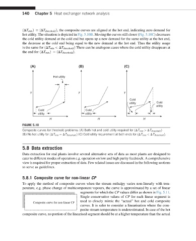
ðDT min Þ¼ ðDT threshold Þ, the composite curves are aligned at the hot end, indicating zero demand for
hot utility. The situation is depicted in Fig. 5.10B. Moving the curves still closer (Fig. 5.10C) decreases
the cold utility demand at the cold end but opens up a new demand for the same utility at the hot end,
the decrease at the cold end being equal to the new demand at the hot end. Thus the utility usage
is the same for ðDT min < DT threshold Þ There can be analogous cases where the cold utility disappears at
the end for ðDT min Þ¼ ðDT threshold Þ.

(A) (B) (C)

Hot utility

T T T

Cold
utility Cold
utility
Cold Cold
utility utility
H H H

FIGURE 5.10
Composite curves for threshold problems: (A) Both hot and cold utility required for ðDT min > DT threshold Þ
(B) No hot utility for ðDT min ¼ DT threshold Þ (C) Cold utility requirement at both ends for ðDT min < DT threshold Þ.

5.8 Data extraction

Data extraction for real plants involve several alternative sets of data as most plants are designed to
cater to different modes of operation e.g. operation on low and high purity feedstock. A comprehensive
view is required for proper extraction of data. Few related issues are discussed in the following sections
to serve as guidelines.

5.8.1 Composite curve for non-linear CP
To apply the method of composite curves when the stream enthalpy varies non-linearly with tem-
perature, e.g. phase change of multicomponent vapours, the curve is approximated by a set of linear
segments for which the CP values differ as shown in Fig. 5.11.
Single conservative values of CP for each linear segment is
used to closely mimic the “actual” hot and cold composite
Composite curve for non-linear CP
curves. It is safer to consider a linearisation where the com-
posite stream temperature is underestimated. In case of the hot
composite curve, no portion of the linearised segment should be at a higher temperature than the actual