Page 147 - Process Equipment and Plant Design Principles and Practices by Subhabrata Ray Gargi Das

144 Chapter 5 Heat exchanger network analysis

200
180 T pinch (140°C)
160
140 Hot composite
T (°C) → 120 composite
Shifted
100
80 curves Cold composite
60
40
20
0 100 200 300 400 500 600 700 800 900
H (kW) →
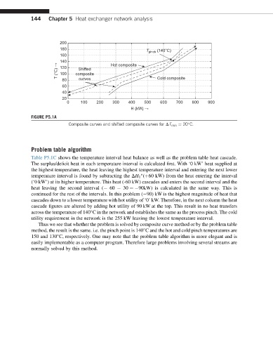
FIGURE P5.1A
Composite curves and shifted composite curves for DT min ¼ 20 C.

Problem table algorithm
Table P5.1C shows the temperature interval heat balance as well as the problem table heat cascade.
The surplus/deficit heat in each temperature interval is calculated first. With ‘0 kW’ heat supplied at
the highest temperature, the heat leaving the highest temperature interval and entering the next lower
temperature interval is found by subtracting the DH 1 (þ60 kW) from the heat entering the interval

(‘0 kW’) at its higher temperature. This heat (-60 kW) cascades and enters the second interval and the
heat leaving the second interval ( 60 30 ¼ 90kW) is calculated in the same way. This is
continued for the rest of the intervals. In this problem ( 90) kW is the highest magnitude of heat that
cascades down to a lower temperature with hot utility of ‘0’ kW. Therefore, in the next column the heat
cascade figures are altered by adding hot utility of 90 kW at the top. This result in no heat transfers
across the temperature of 140 C in the network and establishes the same as the process pinch. The cold

utility requirement in the network is the 255 kW leaving the lowest temperature interval.
Thus we see that whether the problem is solved by composite curve method or by the problem table
method, the result is the same. i.e. the pinch point is 140 C and the hot and cold pinch temperatures are

150 and 130 C, respectively. One may note that the problem table algorithm is more elegant and is

easily implementable as a computer program. Therefore large problems involving several streams are
normally solved by this method.