Page 151 - Process Equipment and Plant Design Principles and Practices by Subhabrata Ray Gargi Das

148 Chapter 5 Heat exchanger network analysis

Area requirement: The area required for each exchanger can be estimated if the numerical values of
the heat transfer coefficients in the last column of Table P5.1A are available. The procedure for area
calculation is provided in Chapter 4.
Solution (B)
Considering multi-level utilities e HP and MP steam are available at 220 and 170 C, respectively,

and cooling water is available at 30 C.

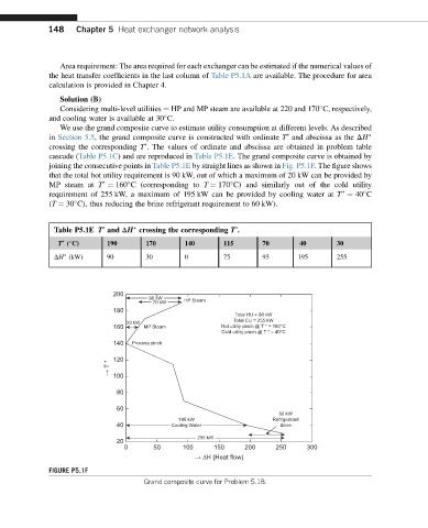
We use the grand composite curve to estimate utility consumption at different levels. As described
in Section 5.5, the grand composite curve is constructed with ordinate T and abscissa as the DH

crossing the corresponding T . The values of ordinate and abscissa are obtained in problem table

cascade (Table P5.1C) and are reproduced in Table P5.1E. The grand composite curve is obtained by
joining the consecutive points in Table P5.1E by straight lines as shown in Fig. P5.1F. The figure shows
that the total hot utility requirement is 90 kW, out of which a maximum of 20 kW can be provided by
MP steam at T ¼ 160 C (corresponding to T ¼ 170 C) and similarly out of the cold utility

requirement of 255 kW, a maximum of 195 kW can be provided by cooling water at T ¼ 40 C

(T ¼ 30 C), thus reducing the brine refrigerant requirement to 60 kW).

Table P5.1E T and DH crossing the corresponding T .

T ( C) 190 170 140 115 70 40 30

DH (kW) 90 30 0 75 93 195 255

200
90 kW
70 kW HP Steam
180
Total HU = 90 kW
Total CU = 255 kW
20 kW
160 MP Steam Hot utility pinch @ T * = 160°C
Cold utility pinch @ T * = 40°C
140 Process pinch
120
→ T * 100

80

60
60 kW
195 kW Refrigerated
40 Cooling Water Brine
255 kW
20
0 50 100 150 200 250 300
→ ΔH (Heat flow)
FIGURE P5.1F
Grand composite curve for Problem 5.1B.